Chapter 30: Limited Labeled Data

Suppose we plot a learning curve (as shown in Figure [fig:ch05-fig01] on page , for example) and find the machine learning model overfits and could benefit from more training data. What are some different approaches for dealing with limited labeled data in supervised machine learning settings?

In lieu of collecting more data, there are several methods related to regular supervised learning that we can use to improve model performance in limited labeled data regimes.

Improving Model Performance with Limited Labeled Data

The following sections explore various machine learning paradigms that help in scenarios where training data is limited.

Labeling More Data

Collecting additional training examples is often the best way to improve the performance of a model (a learning curve is a good diagnostic for this). However, this is often not feasible in practice, because acquiring high-quality data can be costly, computational resources and storage might be insufficient, or the data may be hard to access.

Bootstrapping the Data

Similar to the techniques for reducing overfitting discussed in Chapter [ch05], it can be helpful to “bootstrap” the data by generating modified (augmented) or artificial (synthetic) training examples to boost the performance of the predictive model. Of course, improving the quality of data can also lead to the improved predictive performance of a model, as discussed in Chapter [ch21].

Transfer Learning

Transferlearningdescribestrainingamodelonageneraldataset(forexample, ImageNet) and then fine-tuning the pretrained target dataset (for example, a dataset consisting of different bird species), as outlined in Figure 1.1.

The process of transfer learning

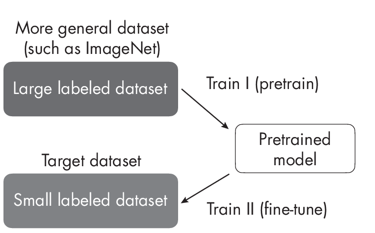
Transfer learning is usually done in the context of deep learning, where model weights can be updated. This is in contrast to tree-based methods, since most decision tree algorithms are nonparametric models that do not support iterative training or parameter updates.

Self-Supervised Learning

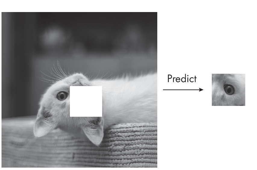
Similar to transfer learning, in self-supervised learning, the model is pretrained on a different task before being fine-tuned to a target task for which only limited data exists. However, self-supervised learning usually relies on label information that can be directly and automatically extracted from unlabeled data. Hence, self-supervised learning is also often called unsupervised pretraining.

Common examples of self-supervised learning include the next word (used in GPT, for example) or masked word (used in BERT, for example) pretraining tasks in language modeling, covered in more detail in Chapter [ch17]. Another intuitive example from computer vision includes inpainting: predicting the missing part of an image that was randomly removed, illustrated in Figure 1.2.

Inpainting for self-supervised learning

For more detail on self-supervised learning, see Chapter [ch02].

Active Learning

In active learning, illustrated in Figure 1.3, we typically involve manual labelers or users for feedback during the learning process. However, instead of labeling the entire dataset up front, active learning includes a prioritization scheme for suggesting unlabeled data points for labeling to maximize the machine learning model’s performance.

In active learning, a model queries an
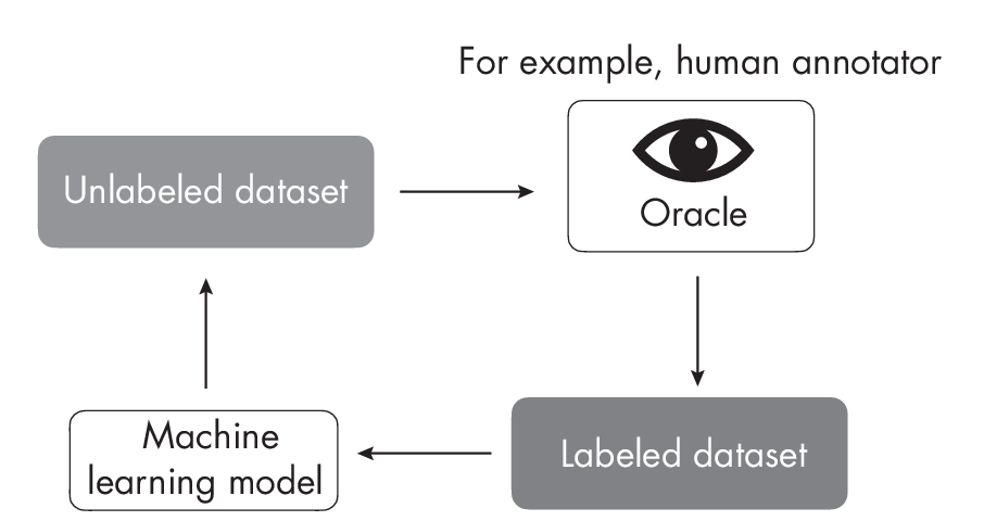
oracle for labels.

The term active learning refers to the fact that the model actively selects data for labeling. For example, the simplest form of active learning selects data points with high prediction uncertainty for labeling by a human annotator (also referred to as an oracle).

Few-Shot Learning

In a few-shot learning scenario, we often deal with extremely small datasets that include only a handful of examples per class. In research contexts, 1-shot(one example per class) and 5-shot (five examples per class) learning scenarios are very common. An extreme case of few-shot learning is zero-shot learning, where no labels are provided. Popular examples of zero-shot learning include GPT-3 and related language models, where the user has to provide all the necessary information via the input prompt, as illustrated in Figure 1.4.

Zero-shot classification with ChatGPT

For more detail on few-shot learning, see Chapter [ch03].

Meta-Learning

Meta-learning involves developing methods that determine how machine learning algorithms can best learn from data. We can therefore think of meta-learning as “learning to learn.” The machine learning community has developed several approaches for meta-learning. Within the machine learning community, the term meta-learning doesn’t just represent multiple subcategories and approaches; it is also occasionally employed to describe related yet distinct processes, leading to nuances in its interpretation and application.

Meta-learning is one of the main subcategories of few-shot learning. Here, the focus is on learning a good feature extraction module, which converts support and query images into vector representations. These vector representations are optimized for determining the predicted class of the query example via comparisons with the training examples in the support set. (This form of meta-learning is illustrated in Chapter [ch03] on page .) Another branch of meta-learning unrelated to the few-shot learning approach is focused on extracting metadata (also called meta-features) from datasets for supervised learning tasks, as illustrated in Figure 1.5. The meta-features are descriptions of the dataset itself. For example, these can include the number of features and statistics of the different features (kurtosis, range, mean, and so on).

The meta-learning process involving the extraction of metadata

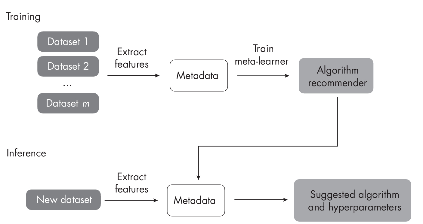
The extracted meta-features provide information for selecting a machine learning algorithm for the dataset at hand. Using this approach, we can narrow down the algorithm and hyperparameter search spaces, which helps reduce overfitting when the dataset is small.

Weakly Supervised Learning

Weakly supervised learning, illustrated in Figure 1.6, involves using an external label source to generate labels for an unlabeled dataset. Often, the labels created by a weakly supervised labeling function are more noisy or inaccurate than those produced by a human or domain expert, hence the term weakly supervised. We can develop or adopt a rule-based classifier to create the labels in weakly supervised learning; these rules usually cover only a subset of the unlabeled dataset.

Weakly supervised learning uses external labeling functions to
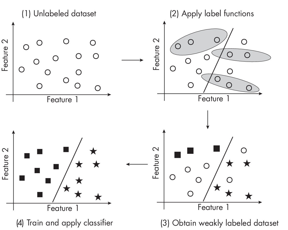
train machine learning models.

Let’sreturntotheexampleofemailspamclassificationfromChapter [ch23] to illustrate a rule-based approach for data labeling. In weak supervision, we could design a rule-based classifier based on the keyword SALE in the email subject header line to identify a subset of spam emails. Note that while we may use this rule to label certain emails as spam positive, we should not apply this rule to label emails without SALE as non-spam. Instead, we should either leave those unlabeled or apply a different rule to them.

There is a subcategory of weakly supervised learning referred to as PU-learning. In PU-learning, which is short for positive-unlabeled learning, we label and learn only from positive examples.

Semi-Supervised Learning

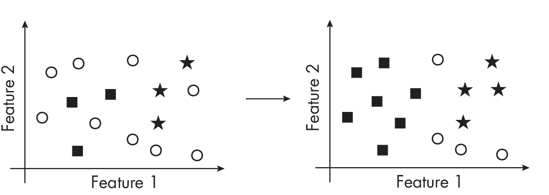
Semi-supervised learning is closely related to weakly supervised learning: it also involves creating labels for unlabeled instances in the dataset. The main difference between these two methods lies in how we create the labels. In weak supervision, we create labels using an external labeling function that is often noisy, inaccurate, or covers only a subset of the data. In semi-supervision, we do not use an external label function; instead, we leverage the structure of the data itself. We can, for example, label additional data points based on the density of neighboring labeled data points, as illustrated in Figure 1.7.

Semi-supervised learning

While we can apply weak supervision to an entirely unlabeled dataset, semi-supervised learning requires at least a portion of the data to be labeled. In practice, it is possible first to apply weak supervision to label a subset of the data and then to use semi-supervised learning to label instances that were not captured by the labeling functions.

Thanks to their close relationship, semi-supervised learning is sometimes referred to as a subcategory of weakly supervised learning, and vice versa.

Self-Training

Self-training falls somewhere between semi-supervised learning and weakly supervised learning. For this technique, we train a model to label the dataset or adopt an existing model to do the same. This model is also referred to as a pseudo-labeler.

Self-training does not guarantee accurate labels and is thus related to weakly supervised learning. Moreover, while we use or adopt a machine learning model for this pseudo-labeling, self-training is also related to semi-supervised learning.

An example of self-training is knowledge distillation, discussed in Chapter [ch06].

Multi-Task Learning

Multi-task learning trains neural networks on multiple, ideally related tasks. For example, if we are training a classifier to detect spam emails, spam classification is the main task. In multi-task learning, we can add one or more related tasks for the model to solve, referred to as auxiliary tasks. For the spam email example, an auxiliary task could be classifying the email’s topic or language.

Typically, multi-task learning is implemented via multiple loss functions that have to be optimized simultaneously, with one loss function for each task. The auxiliary tasks serve as an inductive bias, guiding the model to prioritize hypotheses that can explain multiple tasks. This approach often results in models that perform better on unseen data. There are two subcategories of multi-task learning: multi-task learning with hard parameter sharing and multi-task learning with soft parameter sharing. Figure [fig:ch30-fig08] illustrates the difference between these two methods.

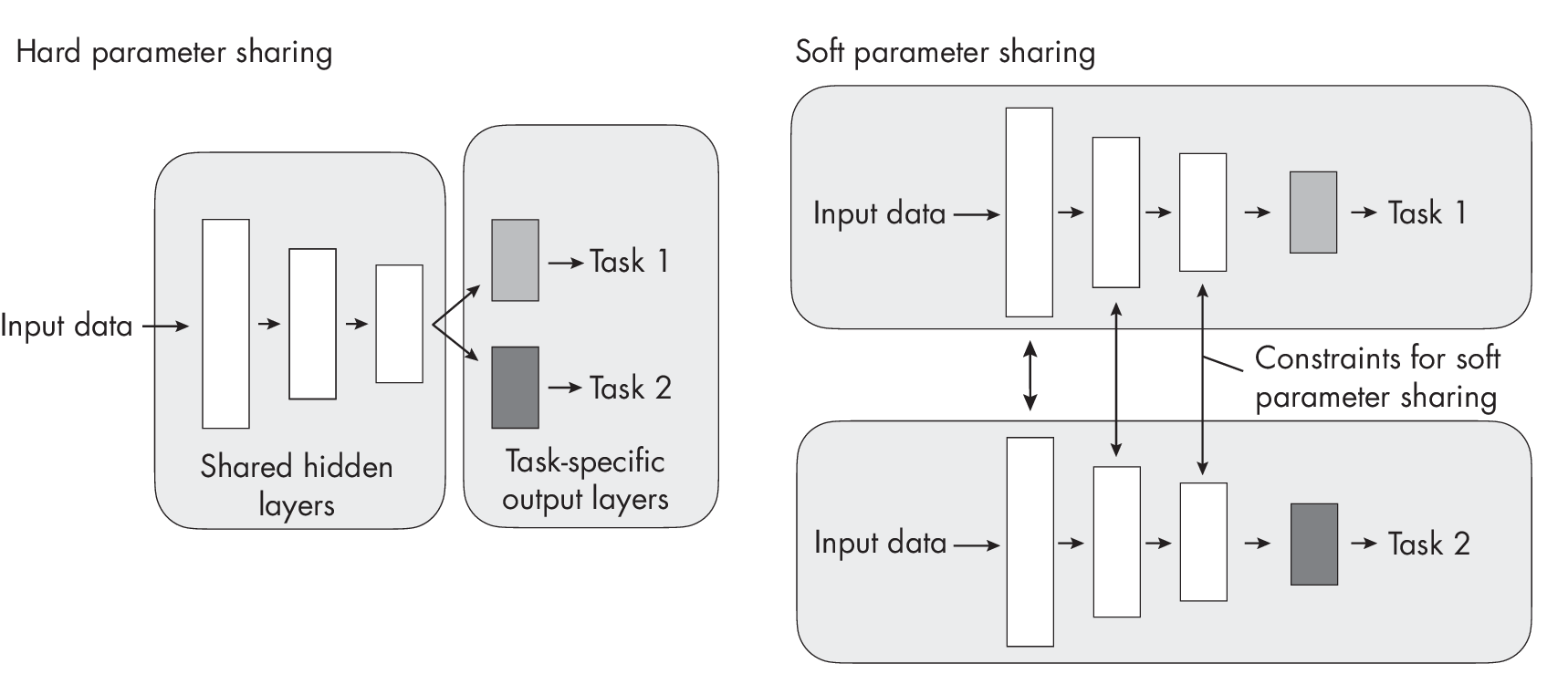
In hard parameter sharing, as shown in Figure [fig:ch30-fig08], only the output layers are task specific, while all the tasks share the same hidden layers and neural network backbone architecture. In contrast, soft parameter sharing uses separate neural networks for each task, but regularization techniques such as distance minimization between parameter layers are applied to encourage similarity among the networks.

Multimodal Learning

While multi-task learning involves training a model with multiple tasks and loss functions, multimodal learning focuses on incorporating multiple types of input data.

Common examples of multimodal learning are architectures that take both image and text data as input (though multimodal learning is not restricted to only two modalities and can be used for any number of input modalities). Depending on the task, we may employ a matching loss that forces the embedding vectors between related images and text to be similar, as shown in Figure 1.8. (See Chapter [ch01] for more on embedding vectors.)

Multimodal learning with a matching loss

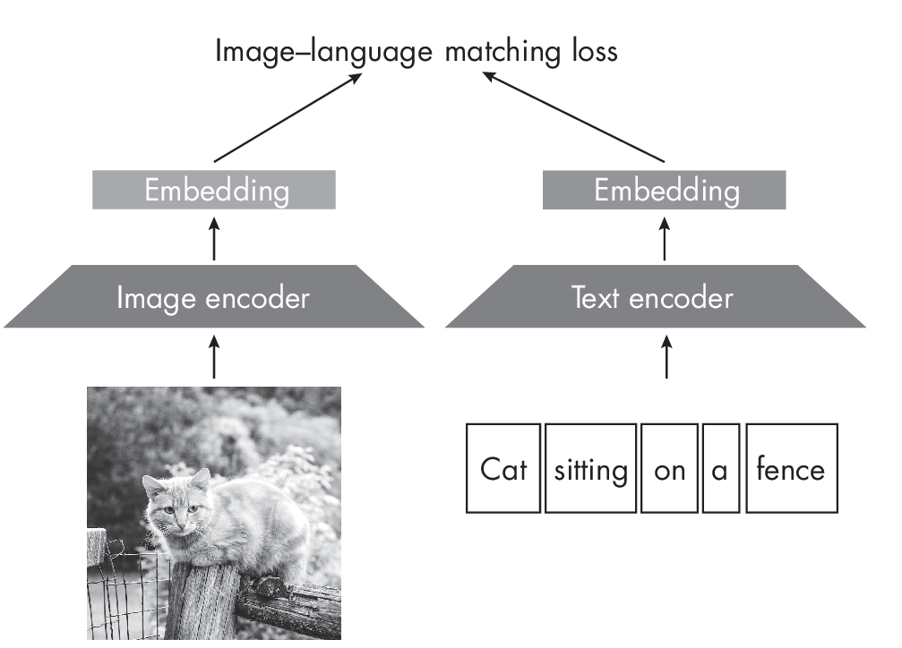
Figure 1.8 shows image and text encoders as separate components. The image encoder can be a convolutional backbone or a vision transformer, and the language encoder can be a recurrent neural network or language transformer. However, it’s common nowadays to use a single transformer-based module that can simultaneously process image and text data. For example, the VideoBERT model has a joint module that processes both video and text for action classification and video captioning.

Optimizing a matching loss, as shown in Figure 1.8, can be useful for learning embeddings that can be applied to various tasks, such as image classification or summarization. However, it is also possible to directly optimize the target loss, like classification or regression, as Figure 1.9 illustrates.

Multimodal learning for optimizing a supervised
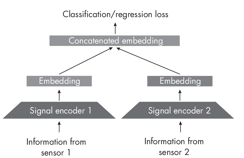
learning objective

Figure 1.9 shows data being collected from two different sensors. One could be a thermometer and the other could be a video camera. The signal encoders convert the information into embeddings (sharing the same number of dimensions), which are then concatenated to form the input representation for the model.

Intuitively, models that combine data from different modalities generally perform better than unimodal models because they can leverage more information. Moreover, recent research suggests that the key to the sucess of multimodal learning is the improved quality of the latent space representation.

Inductive Biases

Choosing models with stronger inductive biases can help lower data requirements by making assumptions about the structure of the data. For example, due to their inductive biases, convolutional networks require less data than vision transformers, as discussed in Chapter [ch13].

Recommendations

Of all these techniques for reducing data requirements, how should we decide which ones to use in a given situation?

Techniques like collecting more data, data augmentation, and feature engineering are compatible with all the methods discussed in this chapter. Multi-task learning and multimodal inputs can also be used with the learning strategies outlined here. If the model suffers from overfitting, we should also include techniques discussed in Chapters [ch05] and [ch06].

But how can we choose between active learning, few-shot learning, transfer learning, self-supervised learning, semi-supervised learning, and weakly supervised learning? Deciding which supervised learning technique(s) to try is highly context dependent. You can use the diagram in Figure 1.10 as a guide to choosing the best method for your particular project.

Recommendations for choosing a supervised learning
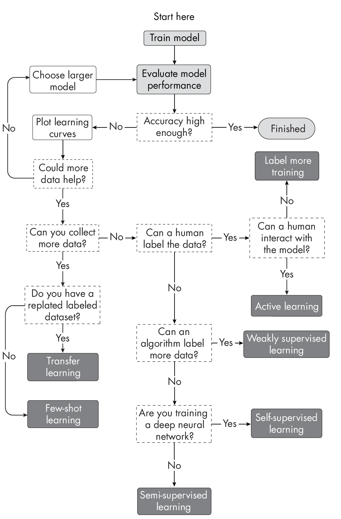
technique

Note that the dark boxes in Figure 1.10 are not terminal nodes but arc back to the second box, “Evaluate model performance”; additional arrows were omitted to avoid visual clutter.

Exercises

30-1. Suppose we are given the task of constructing a machine learning model that utilizes images to detect manufacturing defects on the outer shells of tablet devices similar to iPads. We have access to millions of images of various computing devices, including smartphones, tablets, and computers, which are not labeled; thousands of labeled pictures of smartphones depicting various types of damage; and hundreds of labeled images specifically related to the target task of detecting manufacturing defects on tablet devices. How could we approach this problem using self-supervised learning or transfer learning?

30-2. In active learning, selecting difficult examples for human inspection and labeling is often based on confidence scores. Neural networks can provide such scores by using the logistic sigmoid or softmax function in the output layer to calculate class-membership probabilities. However, it is widely recognized that deep neural networks exhibit overconfidence on out-of-distribution data, rendering their use in active learning ineffective. What are some other methods to obtain confidence scores using deep neural networks for active learning?

References

• While decision trees for incremental learning are not commonly implemented, algorithms for training decision trees in an itera-  tive fashion do exist: https://en.wikipedia.org/wiki/Incremental _decision_tree.

• Models trained with multi-task learning often outperform models trained on a single task: Rich Caruana, “Multitask Learning” (1997), https://doi.org/10.1023%2FA%3A1007379606734.

• A single transformer-based module that can simultaneously process image and text data: Chen Sun et al., “VideoBERT: A Joint Model for Video and Language Representation Learning” (2019), https://arxiv.org/abs/1904.01766.

• The aforementioned research suggesting the key to the success of multimodal learning is the improved quality of the latent space representation: Yu Huang et al., “What Makes Multi-Modal Learning Better Than Single (Provably)” (2021), https://arxiv.org/abs/2106.04538.

• For more information on active learning: Zhen et al., “A Comparative Survey of Deep Active Learning” (2022), https://arxiv.org/abs/2203.13450.

• For a more detailed discussion on how out-of-distribution data can lead to overconfidence in deep neural networks: Anh Nguyen, Jason Yosinski, and Jeff Clune, “Deep Neural Networks Are Easily Fooled: High Confidence Predictions for Unrecognizable Images” (2014), https://arxiv.org/abs/1412.1897.