Chapter 27: Proper Metrics

What are the three properties of a distance function that make it a proper metric?

Metrics are foundational to mathematics, computer science, and various other scientific domains. Understanding the fundamental properties that define a good distance function to measure distances or differences between points or datasets is important. For instance, when dealing with functions like loss functions in neural networks, understanding whether they behave like proper metrics can be instrumental in knowing how optimization algorithms will converge to a solution.

This chapter analyzes two commonly utilized loss functions, the mean squared error and the cross-entropy loss, to demonstrate whether they meet the criteria for proper metrics.

The Criteria

To illustrate the criteria of a proper metric, consider two vectors or points v and w and their distance d(v, w), as shown in Figure 1.1.

The Euclidean distance between two 2D vectors

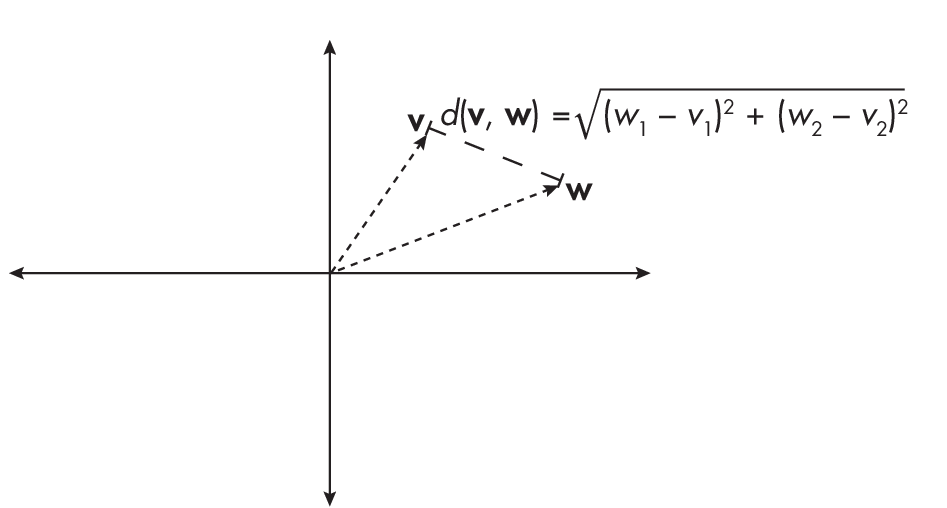
The criteria of a proper metric are the following:

• The distance between two points is always non-negative, d(v, w) \(\geq\) 0, and can be 0 only if the two points are identical, that is, v = w.

• The distance is symmetric; for instance, d(v, w) = d(w, v).

• The distance function satisfies the triangle inequality for any three points: v, w, x, meaning d(v, w) \(\leq\) d(v, x) + d(x, w).

To better understand the triangle inequality, think of the points as vertices of a triangle. If we consider any triangle, the sum of two of the sides is always larger than the third side, as illustrated in Figure 1.2.

Triangle inequality

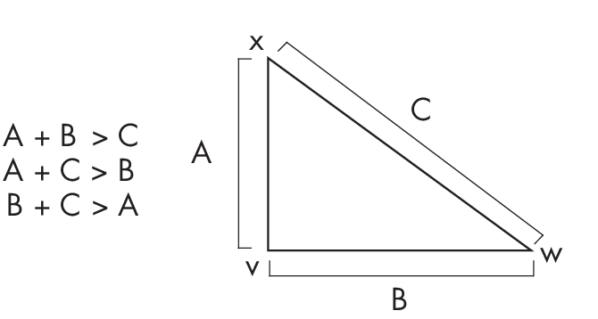
Considerwhatwouldhappenifthetriangleinequalitydepictedin Figure 1.2 weren’t true. If the sum of the lengths of sides AB and BC was shorter than AC, then sides AB and BC would not meet to form a triangle; instead, they would fall short of each other. Thus, the fact that they meet and form a triangle demonstrates the triangle inequality.

The Mean Squared Error

The mean squared error (MSE) loss computes the squared Euclidean distance between a target variable y and a predicted target value \(\hat{\text{\emph{y}}}\):

$$ \mathrm{MSE}=\frac{1}{n} \sum_{i\,=\,1}^n\left(y^{(i)} - \hat{y}^{(i)}\right)^2

The index i denotes the ith data point in the dataset or sample. Is this loss function a proper metric?

For simplicity’s sake, we will consider the squared error (SE) loss between two data points (though the following insights also hold for the MSE). As shown in the following equation, the SE loss quantifies the squared difference between the predicted and actual values for a single data point, while the MSE loss averages these squared differences over all data points in a dataset:

\[\mathrm{SE}(y, \hat{y})=\left(y - \hat{y}\right)^2\]

In this case, the SE satisfies the first part of the first criterion: the distance between two points is always non-negative. Since we are raising the difference to the power of 2, it cannot be negative.

How about the second criterion, that the distance can be 0 only if the two points are identical? Due to the subtraction in the SE, it is intuitive to see that it can be 0 only if the prediction matches the target variable, y = \(\hat{\text{\emph{y}}}\). As with the first criterion, we can use the square to confirm that SE satisfies the second criterion: we have (y – \(\hat{\text{\emph{y}}}\))² = (\(\hat{\text{\emph{y}}}\) – y)².

At first glance, it seems that the squared error loss also satisfies the third criterion, the triangle inequality. Intuitively, you can check this by choosing three arbitrary numbers, here 1, 2, 3:

• (1 – 2)² \(\leq\) (1 – 3)² + (2 – 3)²

• (1 – 3)² \(\leq\) (1 – 2)² + (2 – 3)²

• (2 – 3)² \(\leq\) (1 – 2)² + (1 – 3)²

However, there are values for which this is not true. For example, consider the values a = 0, b = 2, and c = 1. This gives us d(a, b) = 4, d(a, c) = 1, and d(b, c) = 1, such that we have the following scenario, which violates the triangle inequality:

• (0 – 2)² \(\nleq\) (0 – 1)² + (2 – 1)²

• (2 – 1)² \(\leq\) (0 –1)² + (0 – 2)²

• (0 – 1)² \(\leq\) (0 –2)² + (1 – 2)²

Since it does not satisfy the triangle inequality via the example above, we conclude that the (mean) squared error loss is not a proper metric.

However, if we change the squared error into the root-squared error

\[\sqrt\text{(\emph{y} -- } \hat{\text{\emph{y}}})\textsuperscript{2}\]

the triangle inequality can be satisfied:

\[\sqrt{\text{(0 -- 2)\textsuperscript{2}}} \leq \sqrt{\text{(0 -- 1)\textsuperscript{2} +}} \sqrt{\text{(2 -- 1)\textsuperscript{2}}}\]

You might be familiar with the L₂ distance or Euclidean distance, which is known to satisfy the triangle inequality. These two distance metrics are equivalent to the root-squared error when considering two scalar values.

The Cross-Entropy Loss

Cross entropy is used to measure the distance between two probability distributions. In machine learning contexts, we use the discrete cross-entropy loss (CE) between class label y and the predicted probability p when we train logistic regression or neural network classifiers on a dataset consisting of n training examples:

\[\mathrm{CE}(\mathbf{y}, \mathbf{p}) = -\frac{1}{n} \sum_{i\,=\,1}^n y^{(i)} \times \log \left(p^{(i)}\right)\]

Is this loss function a proper metric? Again, for simplicity’s sake, we will look at the cross-entropy function (H) between only two data points:

\[H(y, p) = - y \times \log(p)\]

The cross-entropy loss satisfies one part of the first criterion: the distance is always non-negative because the probability score is a number in the range [0, 1]. Hence, log(p) ranges between –\(\infty\) and 0. The important part is that the H function includes a negative sign. Hence, the cross entropy ranges between \(\infty\) and 0 and thus satisfies one aspect of the first criterion shown above.

However, the cross-entropy loss is not 0 for two identical points. For example, H(0.9, 0.9) = –0.9 \(\times\) log(0.9) = 0.095.

The second criterion shown above is also violated by the cross-entropy loss because the loss is not symmetric: –y \(\times\) log(p) \(\neq\) –p \(\times\) log(y). Let’s illustrate this with a concrete, numeric example:

• If y = 1 and p = 0.5, then –1 \(\times\) log(0.5) = 0.693.

• If y = 0.5 and p = 1, then –0.5 \(\times\) log(1) = 0.

Finally, the cross-entropy loss does not satisfy the triangle inequality, H(r, p) \(\geq\) H(r, q) + H(q, p). Let’s illustrate this with an example as well. Suppose we choose r = 0.9, p = 0.5, and q = 0.4. We have:

• H(0.9, 0.5) = 0.624

• H(0.9, 0.4) = 0.825

• H(0.4, 0.5) = 0.277

As you can see, 0.624 \(\geq\) 0.825 + 0.277 does not hold here.

In conclusion, while the cross-entropy loss is a useful loss function for training neural networks via (stochastic) gradient descent, it is not a proper distance metric, as it does not satisfy any of the three criteria. ### Exercises

27-1. Suppose we consider using the mean absolute error (MAE) as an alternative to the root mean square error (RMSE) for measuring the performance of a machine learning model, where MAE = \(\frac{\text{1}}{\text{\emph{n}}} \sum_{\text{\emph{i}\,=\,1}}^{\text{\emph{n}}}|\) y⁽ⁱ⁾ – \(\hat{\text{\emph{y}}}\textsuperscript{(\text{\emph{i}})}|\) and RMSE = \(\sqrt{\frac{\text{1}}{\text{\emph{n}}} \sum_{\text{\emph{i}\,=\,1}}^{\text{\emph{n}}}( \emph{\text{y}}\textsuperscript{(\emph{\text{i}})} - \hat{\text{\emph{y}}}\textsuperscript{(\emph{\text{i}})})}^\text{2}\). However, a colleague argues that the MAE is not a proper distance metric in metric space because it involves an absolute value, so we should use the RMSE instead. Is this argument correct?

27-2. Based on your answer to the previous question, would you say that the MAE is better or is worse than the RMSE?