Machine Learning Q and AI
30 Essential Questions and Answers on Machine Learning and AI
By Sebastian Raschka. Free to read.
Published by No Starch Press.
Copyright © 2024-2025 by Sebastian Raschka.

Machine learning and AI are moving at a rapid pace. Researchers and practitioners are constantly struggling to keep up with the breadth of concepts and techniques. This book provides bite-sized bits of knowledge for your journey from machine learning beginner to expert, covering topics from various machine learning areas. Even experienced machine learning researchers and practitioners will encounter something new that they can add to their arsenal of techniques.
📘 Print Book:
Amazon
No Starch Press
📄 Read Online:
Full Book (Free)
Chapter 25: Confidence Intervals
What are the different ways to construct confidence intervals for machine learning classifiers?
There are several ways to construct confidence intervals for machine learning models, depending on the model type and the nature of your data. For instance, some methods are computationally expensive when working with deep neural networks and are thus more suitable to less resource-intensive machine learning models. Others require larger datasets to be reliable.
The following are the most common methods for constructing confidence intervals:
-
Constructing normal approximation intervals based on a test set
-
Bootstrapping training sets
-
Bootstrapping the test set predictions
-
Confidence intervals from retraining models with different random seeds
Before reviewing these in greater depth, let’s briefly review the definition and interpretation of confidence intervals.
Defining Confidence Intervals
A confidence interval is a type of method to estimate an unknown population parameter. A population parameter is a specific measure of a statistical population, for example, a mean (average) value or proportion. By “specific” measure, I mean there is a single, exact value for that parameter for the entire population. Even though this value may not be known and often needs to be estimated from a sample, it is a fixed and definite characteristic of the population. A statistical population, in turn, is the complete set of items or individuals we study.
In a machine learning context, the population could be considered the entire possible set of instances or data points that the model may encounter, and the parameter we are often most interested in is the true generalization accuracy of our model on this population.
The accuracy we measure on the test set estimates the true generalization accuracy. However, it’s subject to random error due to the specific sample of test instances we happened to use. This is where the concept of a confidence interval comes in. A 95 percent confidence interval for the generalization accuracy gives us a range in which we can be reasonably sure that the true generalization accuracy lies.
Forinstance,ifwetake100differentdatasamplesandcomputea 95 percent confidence interval for each sample, approximately 95 of the 100 confidence intervals will contain the true population value (such as the generalization accuracy), as illustrated in Figure [fig:ch25-fig01].
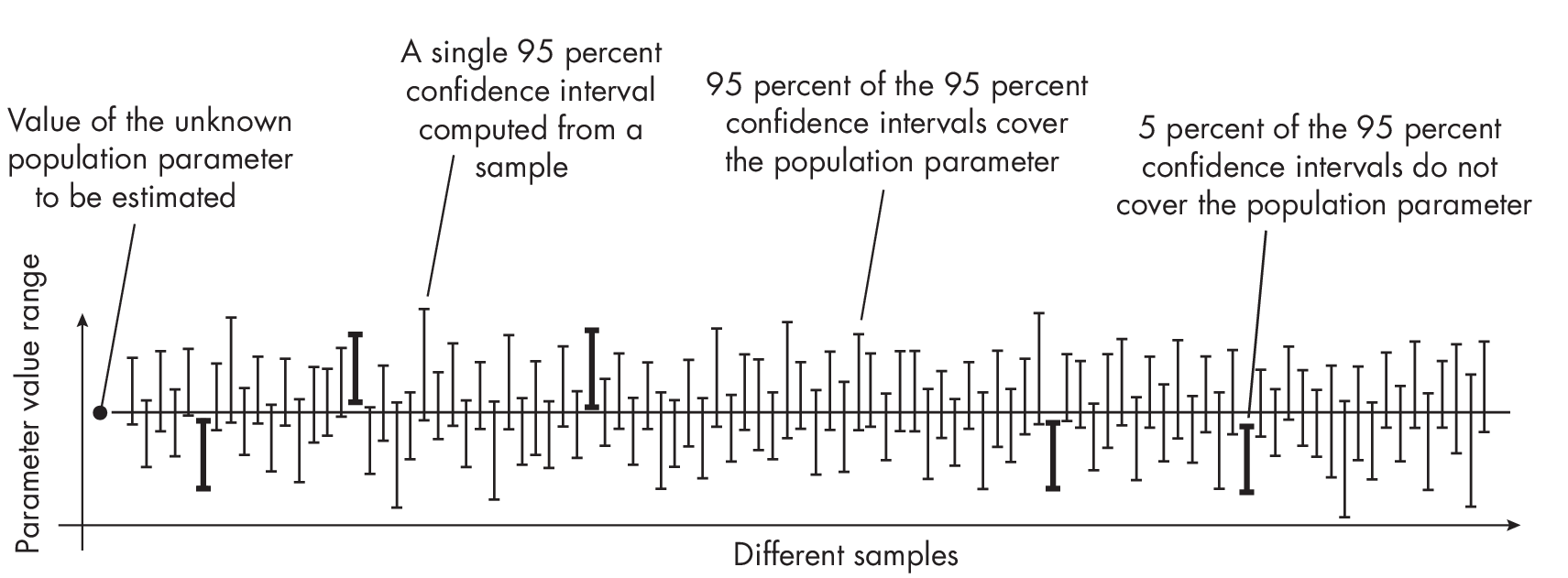
More concretely, if we were to draw 100 different representative test sets from the population (for instance, the entire possible set of instances that the model may encounter) and compute the 95 percent confidence interval for the generalization accuracy from each test set, we would expect about 95 of these intervals to contain the true generalization accuracy.
We can display confidence intervals in several ways. It is common to use a bar plot representation where the top of the bar represents the parameter value (for example, model accuracy) and the whiskers denote the upper andlower levels of the confidence interval (left chart of Figure 1.1). Alternatively, the confidence intervals can be shown without bars, as in the right chart of Figure 1.1.
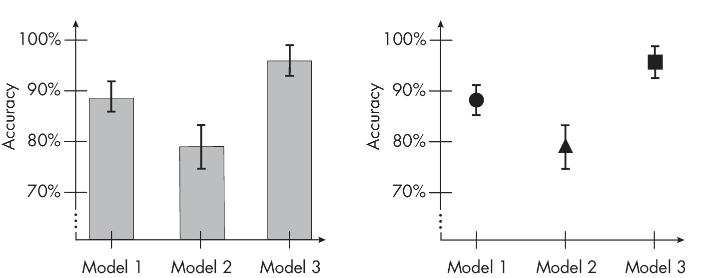
This visualization is functionally useful in a number of ways. For instance, when confidence intervals for two model performances do not overlap, it’s a strong visual indicator that the performances are signifi- cantly different. Take the example of statistical significance tests, such as t-tests: if two 95 percent confidence intervals do not overlap, it strongly suggests that the difference between the two measurements is statistically significant at the 0.05 level.
On the other hand, if two 95 percent confidence intervals overlap, we cannot automatically conclude that there’s no significant difference between the two measurements. Even when confidence intervals overlap, there can still be a statistically significant difference.
Alternatively, to provide more detailed information about the exact quantities, we can use a table view to express the confidence intervals. The two common notations are summarized in Table 1.1.
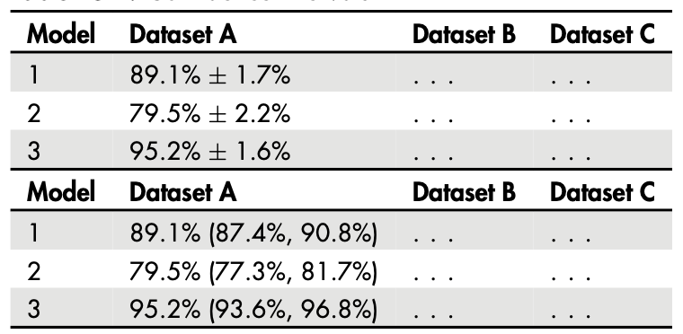
The \(\pm\) notation is often preferred if the confidence interval is symmetric, meaning the upper and lower endpoints are equidistant from the estimated parameter. Alternatively, the lower and upper confidence intervals can be written explicitly.
The Methods
The following sections describe the four most common methods of constructing confidence intervals.
Method 1: Normal Approximation Intervals
The normal approximation interval involves generating the confidence interval from a single train-test split. It is often considered the simplest and most traditional method for computing confidence intervals. This approach is especially appealing in the realm of deep learning, where training models is computationally costly. It’s also desirable when we are interested in evaluating a specific model, instead of models trained on various data partitions like in k-fold cross-validation.
How does it work? In short, the formula for calculating the confidence interval for a predicted parameter (for example, the sample mean, denoted as \(\bar{x}\), assuming a normal distribution, is expressed as \(\bar{x}\) \(\pm\) z \(\times\) SE.
In this formula, z represents the z-score, which indicates a particular value’s number of standard deviations from the mean in a standard normal distribution. SE represents the standard error of the predicted parameter (in this case, the sample mean).
For our scenario, the sample mean, denoted as \(\bar{x}\), corresponds to the test set accuracy, ACCtest, a measure of successful predictions in the context of a binomial proportion confidence interval.
The standard error can be calculated under a normal approximation as follows:
\[\text{SE} = \sqrt{ \frac{1}{n} \text{ACC}_{\text{test}}\left(1- \text{ACC}_{\text{test}}\right)}\]In this equation, n signifies the size of the test set. Substituting the standard error back into the previous formula, we obtain the following:
\[\text{ACC}_{\text{test}} \pm z \sqrt{\frac{1}{n} \text{ACC}_{\text{test}}\left(1- \text{ACC}_{\text{test}}\right)}\]Additional code examples to implement this method can also be found in the supplementary/q25_confidence-intervals subfolder in the supplementary code repository at https://github.com/rasbt/MachineLearning-QandAI-book. While the normal approximation interval method is very popular due to its simplicity, it has some downsides. First, the normal approximation may not always be accurate, especially for small sample sizes or for data that is not normally distributed. In such cases, other methods of computing confidence intervals may be more accurate. Second, using a single train-test split does not provide information about the variability of the model performance across different splits of the data. This can be an issue if the performance is highly dependent on the specific split used, which may be the case if the dataset is small or if there is a high degree of variability in the data.
Method 2: Bootstrapping Training Sets
Confidence intervals serve as a tool for approximating unknown parameters. However, when we are restricted to just one estimate, such as the accuracy derived from a single test set, we must make certain assumptions to make this work. For example, when we used the normal approximation interval described in the previous section, we assumed normally distributed data, which may or may not hold.
In a perfect scenario, we would have more insight into our test set sample distribution. However, this would require access to many independent test datasets, which is typically not feasible. A workaround is the bootstrap method, which resamples existing data to estimate the sampling distribution.
Inamachinelearningcontext,wecantaketheoriginaldatasetanddraw a random sample with replacement. If the dataset has size n and we draw a random sample with replacement of size n, this implies that some data points will likely be duplicated in this new sample, whereas other data points are not sampled at all.We can then repeat this procedure for multiple rounds to obtain multiple training and test sets. This process is known as out-of-bag bootstrapping, illustrated in Figure [fig:ch25-fig04].

Suppose we constructed k training and test sets. We can now take each of these splits to train and evaluate the model to obtain k test set accuracy estimates. Considering this distribution of test set accuracy estimates, we can take the range between the 2.5th and 97.5th percentile to obtain the 95 percent confidence interval, as illustrated in Figure 1.2.
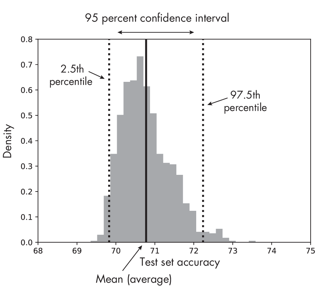
samples, including a 95 percent confidence interval
Unlike the normal approximation interval method, we can consider this out-of-bag bootstrap approach to be more agnostic to the specific distribution. Ideally, if the assumptions for the normal approximation are satisfied, both methodologies would yield identical outcomes.
Since bootstrapping relies on resampling the existing test data, its downside is that it doesn’t bring in any new information that could be available in a broader population or unseen data. Therefore, it may not always be able to generalize the performance of the model to new, unseen data.
Note that we are using the bootstrap sampling approach in this chapter instead of obtaining the train-test splits via k-fold cross-validation, because of the bootstrap’s theoretical grounding via the central limit theorem discussed earlier. There are also more advanced out-of-bag bootstrap methods, such as the .632 and .632+ estimates, which are reweighting the accuracy estimates.
Method 3: Bootstrapping Test Set Predictions
An alternative approach to bootstrapping training sets is to bootstrap test sets.The idea is to train the model on the existing training set as usual and then to evaluate the model on bootstrapped test sets, as illustrated in Figure 1.3. After obtaining the test set performance estimates, we can then apply the percentile method described in the previous section.
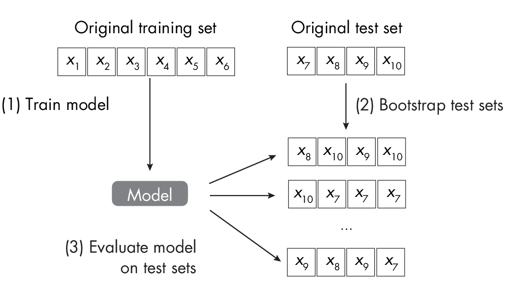
Contrary to the prior bootstrap technique, this method uses a trained model and simply resamples the test set (instead of the training sets). This approach is especially appealing for evaluating deep neural networks, as it doesn’t require retraining the model on the new data splits. However, a disadvantage of this approach is that it doesn’t assess the model’s variability toward small changes in the training data.
Method 4: Retraining Models with Different Random Seeds
In deep learning, models are commonly retrained using various random seeds since some random weight initializations may lead to much better models than others. How can we build a confidence interval from these experiments? If we assume that the sample means follow a normal distribution, we can employ a previously discussed method where we calculate the confidence interval around a sample mean, denoted as \(\bar{x}\), as follows:
\[\bar{x} \pm z \times \text{SE}\]Since in this context we often work with a relatively modest number of samples (for instance, models from 5 to 10 random seeds), assuming a t distribution is deemed more suitable than a normal distribution. Therefore, we substitute the z value with a t value in the preceding formula. (As the sample size increases, the t distribution tends to look more like the standard normal distribution, and the critical values [z and t] become increasingly similar.)
Furthermore,ifweareinterestedintheaverageaccuracy,denoted as \(\overline{\text{ACC}}\)test, we consider ACCtest, j corresponding to a unique random seed j as a sample. The number of random seeds we evaluate would then constitute the sample size n. As such, we would calculate:
\[\overline{\text{ACC}}_{\text{test}} \pm t \times \text{SE}\]Here, SE is the standard error, calculated as SE = SD/\(\!\sqrt{\text{\emph{n}}}\), while
\[\overline{\text{ACC}}_{\text{test}} = \frac{1}{r} \sum_{j\,=\,1}^{r} \text{ACC}_{\text{test}, j}\]is the average accuracy, which we compute over the r random seeds. The standard deviation SD is calculated as follows:
\[\mathrm{SD}=\sqrt{\frac{\sum_j\left(A C C_{\mathrm{test}, j}-\overline{A C C}_{\text {test }}\right)^2}{r-1}}\]To summarize, calculating the confidence intervals using various random seeds is another effective alternative. However, it is primarily beneficial for deep learning models. It proves to be costlier than both the normal approximation approach (method 1) and bootstrapping the test set (method 3), as it necessitates retraining the model. On the bright side, the outcomes derived from disparate random seeds provide us with a robust understanding of the model’s stability.
Recommendations
Each possible method for constructing confidence intervals has its unique advantages and disadvantages. The normal approximation interval is cheap to compute but relies on the normality assumption about the distribution. The out-of-bag bootstrap is agnostic to these assumptions but is substantially more expensive to compute. A cheaper alternative is bootstrapping the test only, but this involves bootstrapping a smaller dataset and may be misleading for small or nonrepresentative test set sizes. Lastly, constructing confidence intervals from different random seeds is expensive but can give us additional insights into the model’s stability.
Exercises
25-1. As mentioned earlier, the most common choice of confidence level is 95 percent confidence intervals. However, 90 percent and 99 percent are also common. Are 90 percent confidence intervals smaller or wider than 95 percent confidence intervals, and why is this the case?
25-2. In “” on page , we created test sets by bootstrapping and then applied the already trained model to compute the test set accuracy on each of these datasets. Can you think of a method or modification to obtain these test accuracies more efficiently?
References
-
A detailed discussion of the pitfalls of concluding statistical significance from nonoverlapping confidence intervals: Martin Krzywinski and Naomi Altman, “Error Bars” (2013), https://www.nature.com/articles/nmeth.2659.
-
A more detailed explanation of the binomial proportion confidence interval: https://en.wikipedia.org/wiki/Binomial_proportion_confidence_interval.
-
For a detailed explanation of normal approximation intervals, see Section 1.7 of my article: “Model Evaluation, Model Selection, and Algorithm Selection in Machine Learning” (2018), https://arxiv.org/abs/1811.12808.
-
Additional information on the central limit theorem for inde- pendent and identically distributed random variables: https://en.wikipedia.org/wiki/Central_limit_theorem.
-
For more on the Berry–Esseen theorem: https://en.wikipedia.org/wiki/Berry–Esseen_theorem.
-
The .632 bootstrap addresses a pessimistic bias of the regular out-of-bag bootstrapping approach: Bradley Efron, “Estimating the Error Rate of a Prediction Rule: Improvement on Cross-Validation” (1983), https://www.jstor.org/stable/2288636.
-
The .632+ bootstrap corrects an optimistic bias introduced in the .632 bootstrap: Bradley Efron and Robert Tibshirani, “Improvements on Cross-Validation: The .632+ Bootstrap Method” (1997), https://www.jstor.org/stable/2965703.
-
A deep learning research paper that discusses bootstrapping the test set predictions: Benjamin Sanchez-Lengeling et al., “Machine Learning for Scent: Learning Generalizable Perceptual Representations of Small Molecules” (2019), https://arxiv.org/abs/1910.10685.
Support the Author
You can support the author in the following ways:
- Subscribe to Sebastian's Substack blog
- Purchase a copy on Amazon or No Starch Press
- Write an Amazon review