Chapter 23: Data Distribution Shifts

What are the main types of data distribution shifts we may encounter after model deployment?

Data distribution shifts are one of the most common problems when putting machine learning and AI models into production. In short, they refer to the differences between the distribution of data on which a model was trained and the distribution of data it encounters in the real world. Often, these changes can lead to significant drops in model performance because the model’s predictions are no longer accurate.

There are several types of distribution shifts, some of which are more problematic than others. The most common are covariate shift, concept drift, label shift, and domain shift; all discussed in more detail in the following sections.

Covariate Shift

Suppose p(x) describes the distribution of the input data (for instance, the features), p(y) refers to the distribution of the target variable (or class label distribution), and p(y\(|\)x) is the distribution of the targets y given the inputs x.

Covariate shift happens when the distribution of the input data, p(x), changes, but the conditional distribution of the output given the input, p(y\(|\)x), remains the same.

Figure 1.1 illustrates covariate shift where both the feature values of the training data and the new data encountered during production follow a normal distribution. However, the mean of the new data has changed from the training data.

Training data and new data distributions differ under covariate shift.

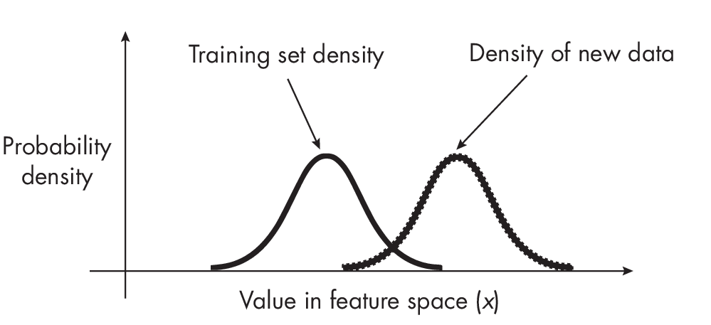
For example, suppose we trained a model to predict whether an email is spam based on specific features. Now, after we embed the email spam filter in an email client, the email messages that customers receive have drastically different features. For example, the email messages are much longer and are sent from someone in a different time zone. However, if the way those features relate to an email being spam or not doesn’t change, then we have a covariate shift.

Covariate shift is a very common challenge when deploying machine learning models. It means that the data the model receives in a live or production environment is different from the data on which it was trained. How-  ever, because the relationship between inputs and outputs, p(y\(|\)x), remains the same under covariate shift, techniques are available to adjust for it.

A common technique to detect covariate shift is adversarial validation, which is covered in more detail in Chapter [ch29]. Once covariate shift is detec-  ted, a common method to deal with it is importance weighting, which assigns different weights to the training example to emphasize or de-emphasize certain instances during training. Essentially, instances that are more likely to appear in the test distribution are given more weight, while instances that are less likely to occur are given less weight. This approach allows the model to focus more on the instances representative of the test data during training, making it more robust to covariate shift.

Label Shift

Label shift, sometimes referred to as prior probability shift, occurs when the class label distribution p(y) changes, but the class-conditional distribution p(y\(|\)x) remains unchanged. In other words, there is a significant change in the label distribution or target variable.

As an example of such a scenario, suppose we trained an email spam classifier on a balanced training dataset with 50 percent spam and 50 percent non-spam email. In contrast, in the real world, only 10 percent of email messages are spam.

A common way to address label shifts is to update the model using the weighted loss function, especially when we have an idea of the new distribution of the labels. This is essentially a form of importance weighting. By adjusting the weights in the loss function according to the new label distribution, we are incentivizing the model to pay more attention to certain classes that have become more common (or less common) in the new data. This helps align the model’s predictions more closely with the current reality, improving its performance on the new data.

Concept Drift

Concept drift refers to the change in the mapping between the input features and the target variable. In other words, concept drift is typically associated with changes in the conditional distribution p(y\(|\)x), such as the relationship between the inputs x and the output y.

Using the example of the spam email classifier from the previous section, the features of the email messages might remain the same, but how those features relate to whether an email is spam might change. This could be due to a new spamming strategy that wasn’t present in the training data. Concept drift can be much harder to deal with than the other distribution shifts discussed so far since it requires continuous monitoring and potential model retraining.

Domain Shift

The terms domain shift and concept drift are used somewhat inconsistently across the literature and are sometimes taken to be interchangeable. In reality, the two are related but slightly different phenomena. Concept drift refers to a change in the function that maps from the inputs to the outputs, specifically to situations where the relationship between features and target variables changes as more data is collected over time.

In domain shift, the distribution of inputs, p(x), and the conditional distribution of outputs given inputs, p(y\(|\)x), both change. This is sometimes also called joint distribution shift due to the joint distribution p(x and y) = p(y\(|\)x) \(\cdot\) p(x). We can thus think of domain shift as a combination of both covariate shift and concept drift. In addition, since we can obtain the marginal distribution p(y) by integrating over the joint distribution p(x, y) over the variable x (mathematically expressed as p(y) = \(\int\)p(x, y) dx), covariate drift and concept shift also imply label shift. (However, exceptions may exist where the change in p(x) compensates for the change in p(y\(|\)x) such that p(y) may not change.) Conversely, label shift and concept drift usually also imply covariate shift.

To return once more to the example of email spam classification, domain shift would mean that the features (content and structure of email) and the relationship between the features and target both change over time. For instance, spam email in 2023 might have different features (new types of phishing schemes, new language, and so forth), and the definition of what constitutes spam might have changed as well. This type of shift would be the most challenging scenario for a spam filter trained on 2020 data, as it would have to adjust to changes in both the input data and the target concept.

Domain shift is perhaps the most difficult type of shift to handle, but monitoring model performance and data statistics over time can help detect domain shifts early. Once they are detected, mitigation strategies include collecting more labeled data from the target domain and retraining or adapting the model.

Types of Data Distribution Shifts

Figure 1.2 provides a visual summary of different types of data shifts in the context of a binary (2-class) classification problem, where the black circles refer to examples from one class and the diamonds refer to examples from another class.

Different types of data shifts in a binary
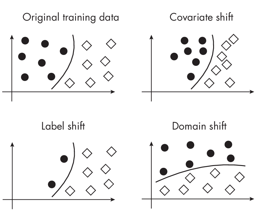
classification context

As noted in the previous sections, some types of distribution shift are more problematic than others. The least problematic among them is typically covariate shift. Here, the distribution of the input features, p(x), changes between the training and testing data, but the conditional distribution of the output given the inputs, p(y\(|\)x), remains constant. Since the underlying relationship between the inputs and outputs remains the same, the model trained on the training data can still apply, in principle, to the testing data and new data.

The most problematic type of distribution shift is typically joint distribution shift, where both the input distribution p(x) and the conditional output distribution p(y\(|\)x) change. This makes it particularly difficult for a model to adjust, as the learned relationship from the training data may no longer hold. The model has to cope with both new input patterns and new rules for making predictions based on those patterns.

However, the “severity” of a shift can vary widely depending on the real-world context. For example, even a covariate shift can be extremely problematic if the shift is severe or if the model cannot adapt to the new input distribution. On the other hand, a joint distribution shift might be manageable if the shift is relatively minor or if we have access to a sufficient amount of labeled data from the new distribution to retrain our model.

In general, it’s crucial to monitor our models’ performance and be aware of potential shifts in the data distribution so that we can take appropriate action if necessary.

Exercises

23-1. What is the big issue with importance weighting as a technique to mitigate covariate shift?

23-2. How can we detect these types of shifts in real-world scenarios, especially when we do not have access to labels for the new data?

References

• Recommendations and pointers to advanced mitigation techniques for avoiding domain shift: Abolfazl Farahani et al., “A Brief Review of Domain Adaptation” (2020), https://arxiv.org/abs/2010.03978.