Chapter 13: Large Training Sets for Vision Transformers

Why do vision transformers (ViTs) generally require larger training sets than convolutional neural networks (CNNs)?

Each machine learning algorithm and model encodes a particular set of assumptions or prior knowledge, commonly referred to as inductive biases, in its design. Some inductive biases are workarounds to make algorithms computationally more feasible, other inductive biases are based on domain knowledge, and some inductive biases are both.

CNNs and ViTs can be used for the same tasks, including image classification, object detection, and image segmentation. CNNs are mainly composed of convolutional layers, while ViTs consist primarily of multi-head attention blocks (discussed in Chapter [ch08] in the context of transformers for natural language inputs).

CNNs have more inductive biases that are hardcoded as part of the algorithmic design, so they generally require less training data than ViTs. In a sense, ViTs are given more degrees of freedom and can or must learn certain inductive biases from the data (assuming that these biases are conducive to optimizing the training objective). However, everything that needs to be learned requires more training examples.

The following sections explain the main inductive biases encountered in CNNs and how ViTs work well without them.

Inductive Biases in CNNs

The following are the primary inductive biases that largely define how CNNs function:

Local connectivity In CNNs, each unit in a hidden layer is connected to only a subset of neurons in the previous layer. We can justify this restriction by assuming that neighboring pixels are more relevant to each other than pixels that are farther apart. As an intuitive example, consider how this assumption applies to the context of recognizing edges or contours in an image.

Weight sharing Via the convolutional layers, we use the same small set of weights (the kernels or filters) throughout the whole image. This reflects the assumption that the same filters are useful for detecting the same patterns in different parts of the image.

Hierarchical processing CNNs consist of multiple convolutional layers to extract features from the input image. As the network progresses from the input to the output layers, low-level features are successively combined to form increasingly complex features, ultimately leading to the recognition of more complex objects and shapes. Furthermore, the convolutional filters in these layers learn to detect specific patterns and features at different levels of abstraction.

Spatial invariance CNNs exhibit the mathematical property of spatial invariance, meaning the output of a model remains consistent even if the input signal is shifted to a different location within the spatial domain. This characteristic arises from the combination of local connectivity, weight sharing, and the hierarchical architecture mentioned earlier.

The combination of local connectivity, weight sharing, and hierarchical processing in a CNN leads to spatial invariance, allowing the model to recognize the same pattern or feature regardless of its location in the input image.

Translation invariance is a specific case of spatial invariance in which the output remains the same after a shift or translation of the input signal in the spatial domain. In this context, the emphasis is solely on moving an object to a different location within an image without any rotations or alterations of its other attributes.

In reality, convolutional layers and networks are not truly translation-invariant; rather, they achieve a certain level of translation equivariance. What is the difference between translation invariance and equivariance? Translation invariance means that the output does not change with an input shift, while translation equivariance implies that the output shifts with the input in a corresponding manner. In other words, if we shift the input object to the right, the results will correspondingly shift to the right, as illustrated in Figure 1.1.

Equivariance under different image translations

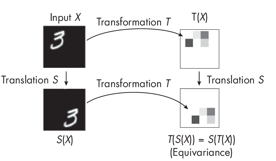
As Figure 1.1 shows, under translation invariance, we get the same output pattern regardless of the order in which we apply the operations: transformation followed by translation or translation followed by transformation.

As mentioned earlier, CNNs achieve translation equivariance through a combination of their local connectivity, weight sharing, and hierarchical processing properties. Figure 1.2 depicts a convolutional operation to illustrate the local connectivity and weight-sharing priors. This figure demonstrates the concept of translation equivariance in CNNs, in which a convolutional filter captures the input signal (the two dark blocks) irrespective of where it is located in the input.

Convolutional filters and translation equivariance

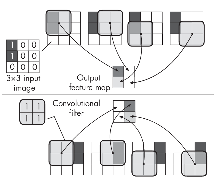
Figure 1.2 shows a \(3 \times 3\) input image that consists of two nonzero pixel values in the upper-left corner (top portion of the figure) or upper-right corner (bottom portion of the figure). If we apply a \(2 \times 2\) convolutional filter to these two input image scenarios, we can see that the output feature maps contain the same extracted pattern, which is on either the left (top of the figure) or the right (bottom of the figure), demonstrating the translation equivariance of the convolutional operation.

For comparison, a fully connected network such as a multilayer perceptron lacks this spatial invariance or equivariance. To illustrate this point, picture a multilayer perceptron with one hidden layer. Each pixel in the input image is connected with each value in the resulting output. If we shift the input by one or more pixels, a different set of weights will be activated, as illustrated in Figure 1.3.

Location-specific weights in fully
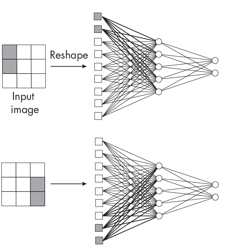
connected layers

Like fully connected networks, ViT architecture (and transformer architecture in general) lacks the inductive bias for spatial invariance or equi-  variance. For instance, the model produces different outputs if we place the same object in two different spatial locations within an image. This is not ideal, as the semantic meaning of an object (the concept that an object represents or conveys) remains the same based on its location. Consequently, it must learn these invariances directly from the data. To facilitate learning useful patterns present in CNNs requires pretraining over a larger dataset.

A common workaround for adding positional information in ViTs is to use relative positional embeddings (also known as relative positional encodings) that consider the relative distance between two tokens in the input sequence. However, while relative embeddings encode information that helps transformers keep track of the relative location of tokens, the transformer still needs to learn from the data whether and how far spatial information is relevant for the task at hand.

ViTs Can Outperform CNNs

The hardcoded assumptions via the inductive biases discussed in previous sections reduce the number of parameters in CNNs substantially compared to fully connected layers. On the other hand, ViTs tend to have larger numbers of parameters than CNNs, which require more training data. (Refer to Chapter [ch11] for a refresher on how to precisely calculate the number of parameters in fully connected and convolutional layers.)

ViTs may underperform compared to popular CNN architectures without extensive pretraining, but they can perform very well with a sufficiently large pretraining dataset. In contrast to language transformers, where unsupervised pretraining (such as self-supervisedlearning, disussed in Chapter [ch02]) is a preferred choice, vision transformers are often pretrained using large, labeled datasets like ImageNet, which provides millions of labeled images for training, and regular supervised learning.

An example of ViTs surpassing the predictive performance of CNNs, given enough data, can be observed from initial research on the ViT architecture, as shown in the paper “An Image Is Worth 16x16 Words: Transformers for Image Recognition at Scale.” This study compared ResNet, a type of convolutional network, with the original ViT design using different dataset sizes for pretraining. The findings also showed that the ViT model excelled over the convolutional approach only after being pretrained on a minimum of 100 million images.

Inductive Biases in ViTs

ViTs also possess some inductive biases. For example, vision transformers patchify the input image to process each input patch individually. Here, each patch can attend to all other patches so that the model learns relationships between far-apart patches in the input image, as illustrated in Figure 1.4.

How a vision transformer operates on image patches

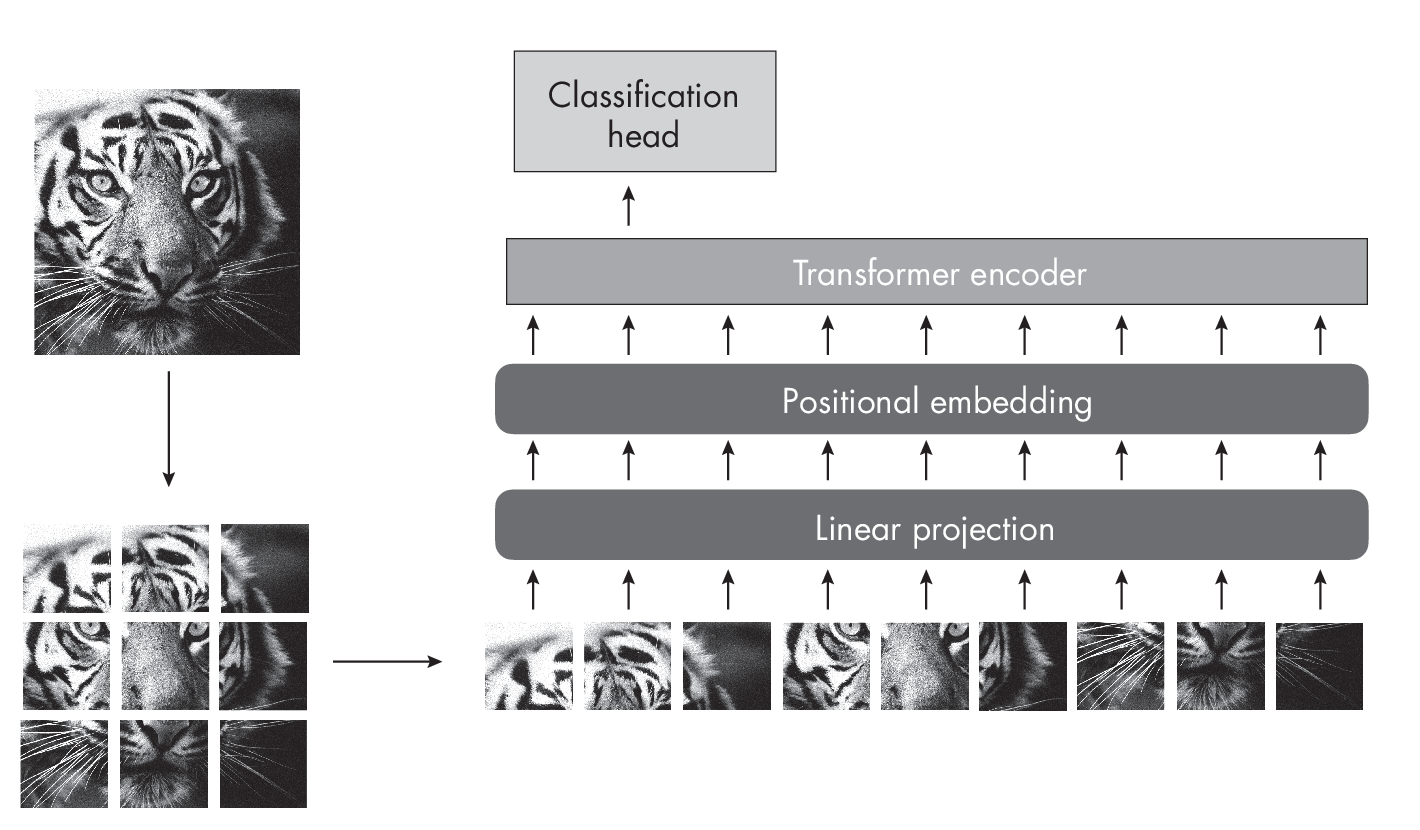
The patchify inductive bias allows ViTs to scale to larger image sizes without increasing the number of parameters in the model, which can be computationally expensive. By processing smaller patches individually, ViTs can efficiently capture spatial relationships between image regions while benefiting from the global context captured by the self-attention mechanism.

This raises another question: how and what do ViTs learn from the training data? ViTs learn more uniform feature representations across all layers, with self-attention mechanisms enabling early aggregation of global information. In addition, the residual connections in ViTs strongly propagate features from lower to higher layers, in contrast to the more hierarchical structure of CNNs.

ViTs tend to focus more on global than local relationships because their self-attention mechanism allows the model to consider long-range dependencies between different parts of the input image. Consequently, the self-attention layers in ViTs are often considered low-pass filters that focus more on shapes and curvature.

In contrast, the convolutional layers in CNNs are often considered high-pass filters that focus more on texture. However, keep in mind that convolutional layers can act as both high-pass and low-pass filters, depending on the learned filters at each layer. High-pass filters detect an image’s edges, fine details, and texture, while low-pass filters capture more global, smooth features and shapes. CNNs achieve this by applying convolutional kernels of varying sizes and learning different filters at each layer.

Recommendations

ViTs have recently begun outperforming CNNs if enough data is available for pretraining. However, this doesn’t make CNNs obsolete, as methods such as the popular EfficientNetV2 CNN architecture are less memory and data hungry.

Moreover, recent ViT architectures don’t rely solely on large datasets, parameter numbers, and self-attention. Instead, they have taken inspiration from CNNs and added soft convolutional inductive biases or even complete convolutional layers to get the best of both worlds.

In short, vision transformer architectures without convolutional layers generally have fewer spatial and locality inductive biases than convolutional neuralnetworks. Consequently, vision transformers need to learn data-related concepts such as local relationships among pixels. Thus, vision transformers require more training data to achieve good predictive performance and produce acceptable visual representations in generative modeling contexts.

Exercises

13-1. Consider the patchification of the input images shown in Figure 1.4. The size of the resulting patches controls a computational and predictive performance trade-off. The optimal patch size depends on the application and desired trade-off between computational cost and model performance. Do smaller patches typically result in higher or lower computational costs?

13-2. Following up on the previous question, do smaller patches typically lead to a higher or lower prediction accuracy?

References

• The paper proposing the original vision transformer model: Alexey Dosovitskiy et al., “An Image Is Worth 16x16 Words: Transformers for Image Recognition at Scale” (2020), https://arxiv.org/abs/2010.11929.

• A workaround for adding positional information in ViTs is to use relative positional embeddings: Peter Shaw, Jakob Uszkoreit, and Ashish Vaswani, “Self-Attention with Relative Position Representations” (2018), https://arxiv.org/abs/1803.02155.

• Residual connections in ViTs strongly propagate features from lower to higher layers, in contrast to the more hierarchical structure of CNNs: Maithra Raghu et al., “Do Vision Transformers See Like Convolutional Neural Networks?” (2021), https://arxiv.org/abs/2108.08810.

• AdetailedresearcharticlecoveringtheEfficientNetV2CNNarchitecture:MingxingTanandQuocV.Le,“EfficientNetV2: SmallerMo-  delsandFasterTraining”(2021),https://arxiv.org/abs/2104.00298.

• A ViT architecture that also incorporates convolutional layers: Stéphane d’Ascoli et al., “ConViT: Improving Vision Transform-  ers with Soft Convolutional Inductive Biases” (2021), https://arxiv.org/abs/2103.10697.

• Another example of a ViT using convolutional layers: Haiping Wu et al., “CvT: Introducing Convolutions to Vision Transformers” (2021), https://arxiv.org/abs/2103.15808.