Machine Learning Q and AI
30 Essential Questions and Answers on Machine Learning and AI
By Sebastian Raschka. Free to read.
Published by No Starch Press.
Copyright © 2024-2025 by Sebastian Raschka.

Machine learning and AI are moving at a rapid pace. Researchers and practitioners are constantly struggling to keep up with the breadth of concepts and techniques. This book provides bite-sized bits of knowledge for your journey from machine learning beginner to expert, covering topics from various machine learning areas. Even experienced machine learning researchers and practitioners will encounter something new that they can add to their arsenal of techniques.
📘 Print Book:
Amazon
No Starch Press
📄 Read Online:
Full Book (Free)
Chapter 10: Sources of Randomness
What are the common sources of randomness when training deep neural networks that can cause non-reproducible behavior during training and inference?
When training or using machine learning models such as deep neural networks, several sources of randomness can lead to different results every time we train or run these models, even though we use the same overall settings. Some of these effects are accidental and some are intended. The following sections categorize and discuss these various sources of randomness.
Optional hands-on examples for most of these categories are provided in the supplementary/q10-random-sources subfolder at https://github.com/rasbt/MachineLearning-QandAI-book.
Model Weight Initialization
All common deep neural network frameworks, including TensorFlow and PyTorch, randomly initialize the weights and bias units at each layer by default. This means that the final model will be different every time we start the training. The reason these trained models will differ when we start with different random weights is the nonconvex nature of the loss, as illustrated in Figure 1.1. As the figure shows, the loss will converge to different local minima depending on where the initial starting weights are located.
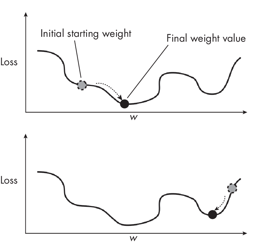
different final weights.
In practice, it is therefore recommended to run the training (if the computational resources permit) at least a handful of times; unlucky initial weights can sometimes cause the model not to converge or to converge to a local minimum corresponding to poorer predictive accuracy.
However, we can make the random weight initialization deterministic by seeding the random generator. For instance, if we set the seed to a specific value like 123, the weights will still initialize with small random values. Nonetheless, the neural network will consistently initialize with the same small random weights, enabling accurate reproduction of results.
Dataset Sampling and Shuffling
When we train and evaluate machine learning models, we usually start by dividing a dataset into training and test sets. This requires random sampling since we have to decide which examples we put into a training set and which examples we put into a test set.
In practice, we often use model evaluation techniques such as k-fold cross-validation or holdout validation. In holdout validation, we split the training set into training, validation, and test datasets, which are also sampling procedures influenced by randomness. Similarly, unless we use a fixed random seed, we get a different model each time we partition the dataset or tune or evaluate the model using k-fold cross-validation since the training partitions will differ.
Nondeterministic Algorithms
We may include random components and algorithms depending on the architecture and hyperparameter choices. A popular example of this is dropout.
Dropout works by randomly setting a fraction of a layer’s units to zero during training, which helps the model learn more robust and generalized representations. This “dropping out” is typically applied at each training iteration with a probability p, a hyperparameter that controls the fraction of units dropped out. Typical values for p are in the range of 0.2 to 0.8.
To illustrate this concept, Figure 1.2 shows a small neural network where dropout randomly drops a subset of the hidden layer nodes in each forward pass during training.
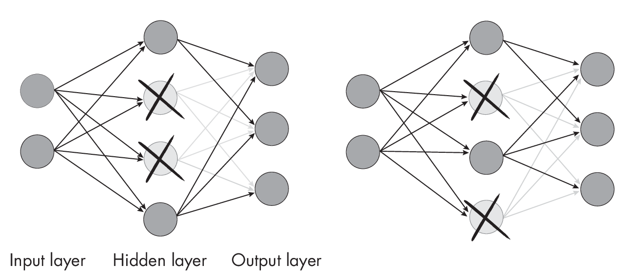
during each forward pass in training.
To create reproducible training runs, we must seed the random gen- erator before training with dropout (analogous to seeding the random generator before initializing the model weights). During inference, we need to disable dropout to guarantee deterministic results. Each deep learning framework has a specific setting for that purpose—a PyTorch example is included in the supplementary/q10-random-sources subfolder at https://github.com/rasbt/MachineLearning-QandAI-book.
Different Runtime Algorithms
The most intuitive or simplest implementation of an algorithm or method is not always the best one to use in practice. For example, when training deep neural networks, we often use efficient alternatives and approximations to gain speed and resource advantages during training and inference.
A popular example is the convolution operation used in convolutional neural networks. There are several possible ways to implement the convolution operation:
The classic direct convolution The common implementation of discrete convolution via an element-wise product between the input and the window, followed by summing the result to get a single number. (See Chapter [ch12] for a discussion of the convolution operation.)
FFT-based convolution Uses fast Fourier transform (FFT) to convert the convolution into an element-wise multiplication in the frequency domain.
Winograd-based convolution
An efficient algorithm for small filter sizes (like
3$\times$3) that reduces the number of multiplications
required for the convolution.
Different convolution algorithms have different trade-offs in terms of memory usage, computational complexity, and speed. By default, libraries such as the CUDA Deep Neural Network library (cuDNN), which are used in PyTorch and TensorFlow, can choose different algorithms for performing convolution operations when running deep neural networks on GPUs. However, the deterministic algorithm choice has to be explicitly enabled. In PyTorch, for example, this can be done by setting
torch.use_deterministic_algorithms(True)
While these approximations yield similar results, subtle numerical differences can accumulate during training and cause the training to converge to slightly different local minima.
Hardware and Drivers
Training deep neural networks on different hardware can also produce different results due to small numeric differences, even when the same algorithms are used and the same operations are executed. These differences may sometimes be due to different numeric precision for floating-point operations. However, small numeric differences may also arise due to hardware and software optimization, even at the same precision.
For instance, different hardware platforms may have specialized optimizations or libraries that can slightly alter the behavior of deep learning algorithms. To give one example of how different GPUs can produce different modeling results, the following is a quotation from the official NVIDIA documentation: “Across different architectures, no cuDNN routines guarantee bit-wise reproducibility. For example, there is no guarantee of bit-wise reproducibility when comparing the same routine run on NVIDIA Volta™ and NVIDIA Turing™ [. . .] and NVIDIA Ampere architecture.”
Randomness and Generative AI
Besides the various sources of randomness mentioned earlier, certain models may also exhibit random behavior during inference that we can think of as “randomness by design.” For instance, generative image and language models may create different results for identical prompts to produce a diverse sample of results. For image models, this is often so that users canselect the most accurate and aesthetically pleasing image. For language models, this is often to vary the responses, for example, in chat agents, to avoid repetition.
The intended randomness in generative image models during inference is often due to sampling different noise values at each step of the reverse process. In diffusion models, a noise schedule defines the noise variance added at each step of the diffusion process.
Autoregressive LLMs like GPT tend to create different outputs for the same input prompt (GPT will be discussed at greater length in Chapters [ch14] and [ch17]). The ChatGPT user interface even has a Regenerate Response button for that purpose. The ability to generate different results is due to the sampling strategies these models employ. Techniques such as top-k sampling, nucleus sampling, and temperature scaling influence the model’s output by controlling the degree of randomness. This is a feature, not a bug, since it allows for diverse responses and prevents the model from producing overly deterministic or repetitive outputs. (See Chapter [ch09] for a more in-depth overview of generative AI and deep learning models; see Chapter [ch17] for more detail on autoregressive LLMs.)
Top-k sampling, illustrated in Figure 1.3, works by sampling tokens from the top k most probable candidates at each step of the next-word generation process.
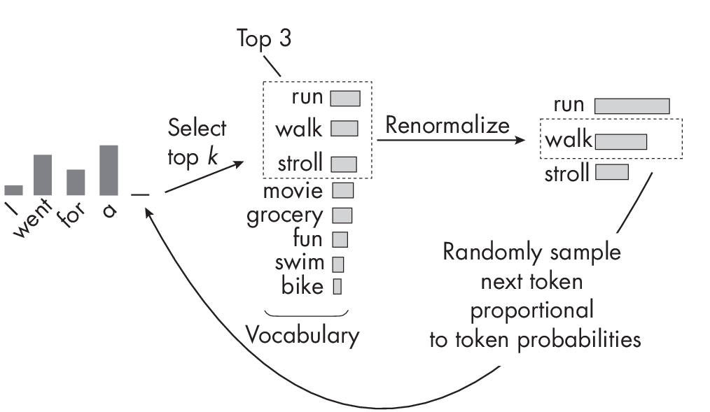
Given an input prompt, the language model produces a probability distribution over the entire vocabulary (the candidate words) for the next token. Each token in the vocabulary is assigned a probability based on the model’s understanding of the context. The selected top-k tokens are then renormalized so that the probabilities sum to 1. Finally, a token is sampled from the renormalized top-k probability distribution and is appended to the input prompt. This process is repeated for the desired length of the generated text or until a stop condition is met.
Nucleus sampling (also known as top-p sampling), illustrated in Figure 1.4, is an alternative to top-k sampling.
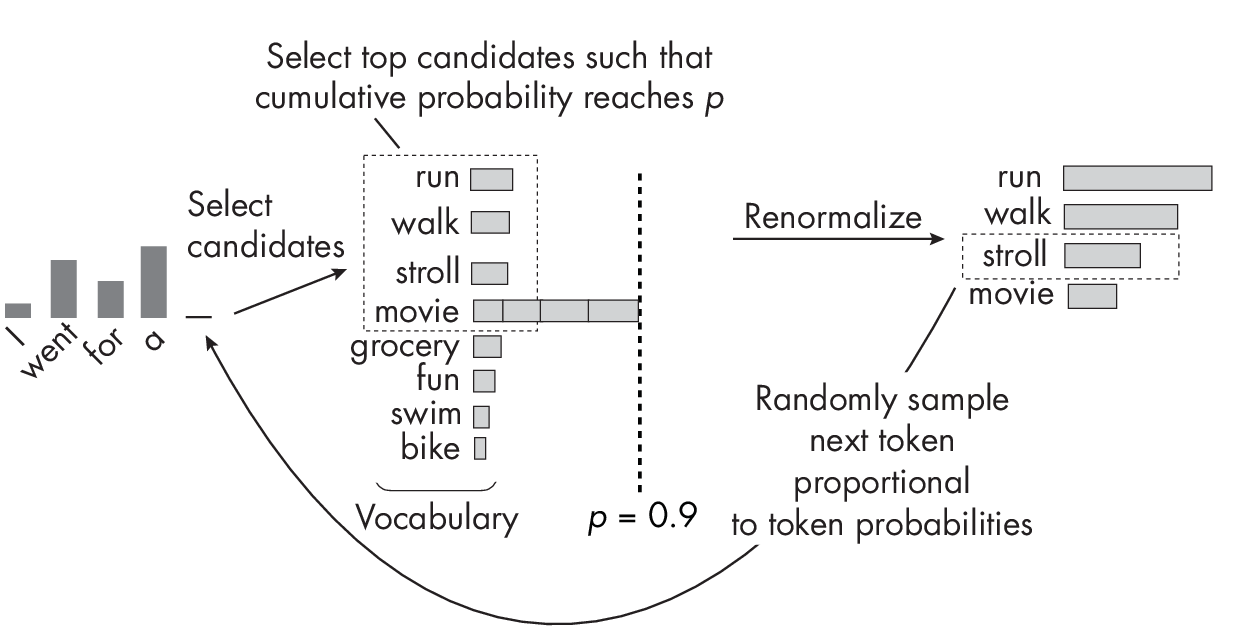
Similar to top-k sampling, the goal of nucleus sampling is to balance diversity and coherence in the output. However, nucleus and top-k sampling differ in how to select the candidate tokens for sampling at each step of the generation process. Top-k sampling selects the k most probable tokens from the probability distribution produced by the language model, regardless of their probabilities. The value of k remains fixed throughout the generation process. Nucleus sampling, on the other hand, selects tokens based on a probability threshold p, as shown in Figure 1.4. It then accumulates the most probable tokens in descending order until their cumulative probability meets or exceeds the threshold p. In contrast to top-k sampling, the size of the candidate set (nucleus) can vary at each step.
Exercises
10-1. Suppose we train a neural network with top-k or nucleus sampling where k and p are hyperparameter choices. Can we make the model behave deterministically during inference without changing the code?
10-2. In what scenarios might random dropout behavior during inference be desired?
References
-
For more about different data sampling and model evaluation techniques, see my article: “Model Evaluation, Model Selection, and Algorithm Selection in Machine Learning” (2018), https://arxiv.org/abs/1811.12808.
-
The paper that originally proposed the dropout technique: Nitish Srivastavaetal.,“Dropout:ASimpleWaytoPreventNeuralNet- works from Overfitting” (2014), https://jmlr.org/papers/v15/sriva stava14a.html.
-
A detailed paper on FFT-based convolution: Lu Chi, Borui Jiang, and Yadong Mu, “Fast Fourier Convolution” (2020), https://dl.acm.org/doi/abs/10.5555/3495724.3496100.
-
Details on Winograd-based convolution: Syed Asad Alam et al., “Winograd Convolution for Deep Neural Networks: Efficient Point Selection” (2022), https://arxiv.org/abs/2201.10369.
-
More information about the deterministic algorithm settings in PyTorch: https://pytorch.org/docs/stable/generated/torch.use_deterministic_algorithms.html.
-
For details on the deterministic behavior of NVIDIA graphics cards, see the “Reproducibility” section of the official NVIDIA documentation: https://docs.nvidia.com/deeplearning/cudnn/developer-guide/index.html#reproducibility.
Support the Author
You can support the author in the following ways:
- Subscribe to Sebastian's Substack blog
- Purchase a copy on Amazon or No Starch Press
- Write an Amazon review