Chapter 9: Generative AI Models

What are the popular categories of deep generative models in deep learning (also called generative AI), and what are their respective downsides?

Many different types of deep generative models have been applied to generating different types of media: images, videos, text, and audio. Beyond these types of media, models can also be repurposed to generate domain-specific data, such as organic molecules and protein structures. This chapter will first define generative modeling and then outline each type of generative model and discuss its strengths and weaknesses.

Generative vs. Discriminative Modeling

In traditional machine learning, there are two primary approaches to modeling the relationship between input data (x) and output labels (y): generative models and discriminative models. Generative models aim to capture the underlying probability distribution of the input data p(x) or the joint distribution p(x, y) between inputs and labels. In contrast, discriminative models focus on modeling the conditional distribution p(y\(|\)x) of the labels given the inputs.

A classic example that highlights the differences between these approa-  ches istocomparethenaiveBayesclassifierandthelogisticregressionclassifier. Both classifiers estimate the class label probabilities p(y\(|\)x) and can be used for classification tasks. However, logistic regression is considered a discriminative model because it directly models the conditional probability distribution p(y\(|\)x) of the class labels given the input features without making assumptions about the underlying joint distribution of inputs and labels. Naive Bayes, on the other hand, is considered a generative model because it models the joint probability distribution p(x, y) of the input features x and the output labels y. By learning the joint distribution, a generative model like naive Bayes captures the underlying data generation process, which enables it to generate new samples from the distribution if needed.

Types of Deep Generative Models

When we speak of deep generative models or deep generative AI, we often loosen this definition to include all types of models capable of producing realistic-looking data (typically text, images, videos, and sound). The remainder of this chapter briefly discusses the different types of deep generative models used to generate such data.

Energy-Based Models

Energy-based models (EBMs) are a class of generative models that learn an energy function, which assigns a scalar value (energy) to each data point. Lower energy values correspond to more likely data points. The model is trained to minimize the energy of real data points while increasing the energy of generated data points. ExamplesofEBMsincludedeepBoltzmannmachines(DBMs).Oneoftheearlybreakthroughsindeeplearning,DBMsprovideameanstolearncomplexrepresentationsofdata.Youcanthinkofthemasaformofunsupervisedpretraining,resultinginmodelsthatcanthenbefine-tunedforvarioustasks.

Somewhat similar to naive Bayes and logistic regression, DBMs and multilayer perceptrons (MLPs) can be thought of as generative and discriminative counterparts, with DBMs focusing on capturing the data generation process and MLPs focusing on modeling the decision boundary between classes or mapping inputs to outputs.

ADBMconsistsofmultiplelayersofhiddennodes,asshowninFigure 1.1. As the figure illustrates, along with the hidden layers, there’s usually a visible layer that corresponds to the observable data. This visible layer serves as the input layer where the actual data or features are fed into the network. In addition to using a different learning algorithm than MLPs (contrastive divergence instead of backpropagation), DBMs consist of binary nodes (neurons) instead of continuous ones.

A four-layer deep Boltzmann machine
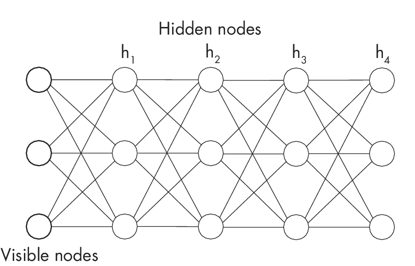
with three stacks of hidden nodes

Suppose we are interested in generating images. A DBM can learn the joint probability distribution over the pixel values in a simple image dataset like MNIST. To generate new images, the DBM then samples from this distribution by performing a process called Gibbs sampling. Here, the visible layer of the DBM represents the input image. To generate a new image, the DBM starts by initializing the visible layer with random values or, alternatively, uses an existing image as a seed. Then, after completing several Gibbs sampling iterations, the final state of the visible layer represents the generated image.

DBMs played an important historical role as one of the first deep generative models, but they are no longer very popular for generating data. They are expensive and more complicated to train, and they have lower expressivity compared to the newer models described in the following sections, which generally results in lower-quality generated samples.

Variational Autoencoders

Variational autoencoders (VAEs) are built upon the principles of variational inference and autoencoder architectures. Variational inference is a method for approximating complex probability distributions by optimizing a simpler, tractable distribution to be as close as possible to the true distribution. Autoencoders are unsupervised neural networks that learn to compress input data into a low-dimensional representation (encoding) and subsequently reconstruct the original data from the compressed representation (decoding) by minimizing the reconstruction error.

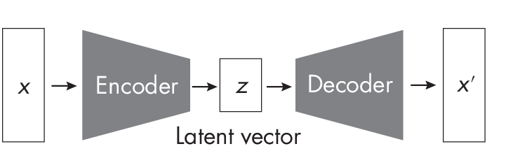
The VAE model consists of two main submodules: an encoder network and a decoder network. The encoder network takes, for example, an input image and maps it to a latent space by learning a probability distribution over the latent variables. This distribution is typically modeled as a Gaus-  sian with parameters (mean and variance) that are functions of the inputimage. The decoder network then takes a sample from the learned latent distribution and reconstructs the input image from this sample. The goal of the VAE is to learn a compact and expressive latent representation that captures the essential structure of the input data while being able to generate new images by sampling from the latent space. (See Chapter [ch01] for more details on latent representations.)

Figure 1.2 illustrates the encoder and decoder submodules of an auto-  encoder, where x\('\) represents the reconstructed input x. In a standard variational autoencoder, the latent vector is sampled from a distribution that approximates a standard Gaussian distribution.

An autoencoder

Training a VAE involves optimizing the model’s parameters to minimize a loss function composed of two terms: a reconstruction loss and a Kullback–Leibler-divergence (KL-divergence) regularization term. The reconstruction loss ensures that the decoded samples closely resemble the input images, while the KL-divergence term acts as a surrogate loss that encourages the learned latent distribution to be close to a predefined prior distribution (usually a standard Gaussian). To generate new images, we then sample points from the latent space’s prior (standard Gaussian) distribution and pass them through the decoder network, which generates new, diverse images that look similar to the training data.

Disadvantages of VAEs include their complicated loss function consisting of separate terms, as well as their often low expressiveness. The latter can result in blurrier images compared to other models, such as generative adversarial networks.

Generative Adversarial Networks

Generative adversarial networks (GANs) are models consisting of interacting subnetworks designed to generate new data samples that are similar to a given set of input data. While both GANs and VAEs are latent variable models that generate data by sampling from a learned latent space, their architectures and learning mechanisms are fundamentally different.

GANs consist of two neural networks, a generator and a discriminator, that are trained simultaneously in an adversarial manner. The generator takes a random noise vector from the latent space as input and generates a synthetic data sample (such as an image). The discriminator’s task is to distinguish between real samples from the training data and fake samples generated by the generator, as illustrated in Figure 1.3.

A generative adversarial network

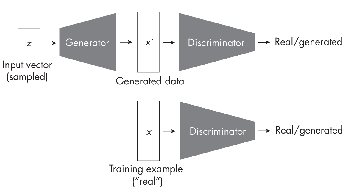
The generator in a GAN somewhat resembles the decoder of a VAE in terms of its functionality. During inference, both GAN generators and VAE decoders take random noise vectors sampled from a known distribution (for example, a standard Gaussian) and transform them into synthetic data samples, such as images.

One significant disadvantage of GANs is their unstable training due to the adversarial nature of the loss function and learning process. Balancing the learning rates of the generator and discriminator can be difficult and can often result in oscillations, mode collapse, or non-convergence. The second main disadvantage of GANs is the low diversity of their generated outputs, often due to mode collapse. Here, the generator is able to fool the discriminator successfully with a small set of samples, which are representative of only a small subset of the original training data.

Flow-Based Models

The core concept of flow-based models, also known as normalizing flows, is inspired by long-standing methods in statistics. The primary goal is to transform a simple probability distribution (like a Gaussian) into a more complex one using invertible transformations.

Althoughtheconceptofnormalizingflowshasbeenapartofthe statistics field for a long time, the implementation of early flow-based deep learning models, particularly for image generation, is a relatively recent development. One of the pioneering models in this area was the non-linear independent components estimation (NICE) approach. NICE begins with a simple probability distribution, often something straightforward like a normal distribution. You can think of this as a kind of “random noise,” or data with no particular shape or structure. NICE then applies a series of transformations to this simple distribution. Each transformation is designed to make the datalook more like the final target (for instance, the distribution of real-world images). These transformations are “invertible,” meaning we can always reverse them back to the original simple distribution. After several successive transformations, the simple distribution has morphed into a complex distribution that closely matches the distribution of the target data (such as images). We can now generate new data that looks like the target data by picking random points from this complex distribution.

Figure 1.4 illustrates the concept of a flow-based model, which maps the complex input distribution to a simpler distribution and back.

A flow-based model

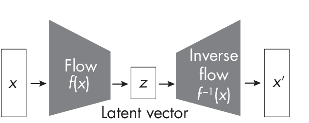
At first glance, the illustration is very similar to the VAE illustration in Figure 1.2. However, while VAEs use neural network encoders like convolutional neural networks, the flow-based model uses simpler decoupling layers, such as simple linear transformations. Additionally, while the decoder in a VAE is independent of the encoder, the data-transforming functions in the flow-based model are mathematically inverted to obtain the outputs.

Unlike VAEs and GANs, flow-based models provide exact likelihoods, which gives us insights into how well the generated samples fit the training data distribution. This can be useful in anomaly detection or density estimation, for example. However, the quality of flow-based models for generating image data is usually lower than GANs. Flow-based models also often require more memory and computational resources than GANs or VAEs since they must store and compute inverses of transformations.

Autoregressive Models

Autoregressive models are designed to predict the next value based on current (and past) values. LLMs for text generation, like ChatGPT (discussed further in Chapter [ch17]), are one popular example of this type of model.

Similar to generating one word at a time, in the context of image gen-  eration, autoregressive models like PixelCNN try to predict one pixel at a time, given the pixels they have seen so far. Such a model might predict pixels from top left to bottom right, in a raster scan order, or in any other defined order.

To illustrate how autoregressive models generate an image one pixel at a time, suppose we have an image of size H\(\times\)W (where H is the height and W is the width), ignoring the color channel for simplicity’s sake. This image consists of N pixels, where i = 1, . . . , N. The probability of observing a particular image in the dataset is then P(Image) = P(i₁, i₂, . . . , i_N). Basedon the chain rule of probability in statistics, we can decompose this joint probability into conditional probabilities:

\begin{aligned}
P( { Image })&=P\left(i_1, i_2, .\,.\,., i_N\right) \\
&=P\left(i_1\right) \cdot P\left(i_2 \mid i_1\right) \cdot P\left(i_3 \mid i_1, i_2\right) \ldots P\left(i_N \mid i_1 \; to \; i_{N-1}\right)
\end{aligned}

Here, P(i₁) is the probability of the first pixel, P(i₂\(|\)i₁) is the probability of the second pixel given the first pixel, P(i₃\(|\)i₁, i₂) is the probability of the third pixel given the first and second pixels, and so on.

In the context of image generation, an autoregressive model essentially tries to predict one pixel at a time, as described earlier, given the pixels it has seen so far. Figure 1.5 illustrates this process, where pixels i₁, . . . , i₅₃ represent the context and pixel i₅₄ is the next pixel to be generated.

Autoregressive
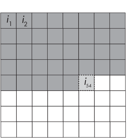
pixel generation

The advantage of autoregressive models is that the next-pixel (or word) prediction is relatively straightforward and interpretable. In addition, auto-  regressive models can compute the likelihood of data exactly, similar to flow-based models, which can be useful for tasks like anomaly detection. Furthermore, autoregressive models are easier to train than GANs as they don’t suffer from issues like mode collapse and other training instabilities.

However, autoregressive models can be slow at generating new samples. This is because they have to generate data one step at a time (for example, pixel by pixel for images), which can be computationally expensive. Auto-  regressive models may also struggle to capture long-range dependencies because each output is conditioned only on previously generated outputs.

In terms of overall image quality, autoregressive models are therefore usually worse than GANs but are easier to train.

Diffusion Models

As discussed in the previous section, flow-based models transform a simple distribution (such as a standard normal distribution) into a complex one (the target distribution) by applying a sequence of invertible and differentiable transformations (flows). Like flow-based models, diffusion models alsoapply a series of transformations. However, the underlying concept is fundamentally different.

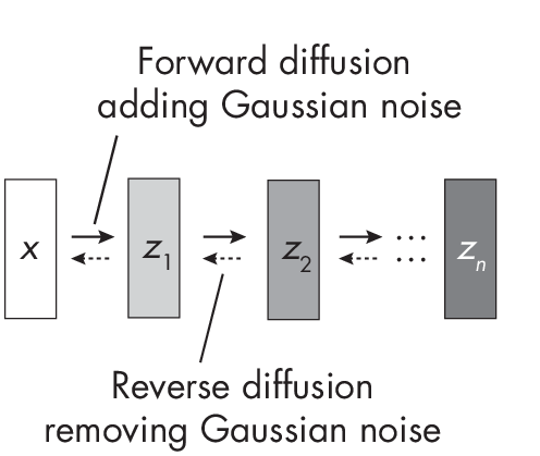
Diffusion models transform the input data distribution into a simple noise distribution over a series of steps using stochastic differential equations. Diffusion is a stochastic process in which noise is progressively added to the data until it resembles a simpler distribution, like Gaussian noise. To generate new samples, the process is then reversed, starting from noise and progressively removing it.

Figure 1.6 outlines the process of adding and removing Gaussian noise from an input image x. During inference, the reverse diffusion process is used to generate a new image x, starting with the noise tensor z_n sampled from a Gaussian distribution.

The diffusion process

While both diffusion models and flow-based models are generative models aiming to learn complex data distributions, they approach the problem from different angles. Flow-based models use deterministic invertible transformations, while diffusion models use the aforementioned stochastic diffusion process.

Recent projects have established state-of-the-art performance in generating high-quality images with realistic details and textures. Diffusion models are also easier to train than GANs. The downside of diffusion models, however, is that they are slower to sample from since they require running a series of sequential steps, similar to flow-based models and autoregressive models.

Consistency Models

Consistency models train a neural network to map a noisy image to a clean one. The network is trained on a dataset of pairs of noisy and clean images and learns to identify patterns in the clean images that are modified by noise. Once the network is trained, it can be used to generate reconstructed images from noisy images in one step.

Consistency model training employs an ordinary differential equation (ODE) trajectory, a path that a noisy image follows as it is gradually denoised. The ODE trajectory is defined by a set of differential equations that describe how the noise in the image changes over time, as illustrated in Figure 1.7.

Trajectories of a consistency model for image
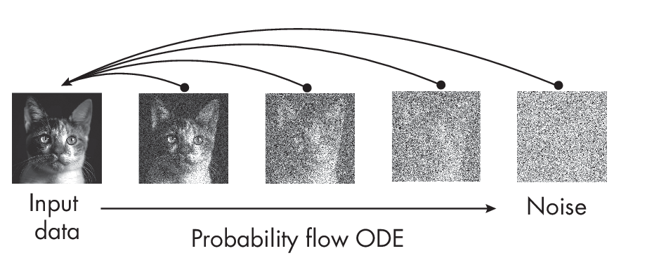
denoising

As Figure 1.7 demonstrates, we can think of consistency models as models that learn to map any point from a probability flow ODE, which smoothly converts data to noise, to the input.

At the time of writing, consistency models are the most recent type of generative AI model. Based on the original paper proposing this method, consistency models rival diffusion models in terms of image quality. Consistency models are also faster than diffusion models because they do not require an iterative process to generate images; instead, they generate images in a single step.

However, while consistency models allow for faster inference, they are still expensive to train because they require a large dataset of pairs of noisy and clean images.

Recommendations

Deep Boltzmann machines are interesting from a historical perspective since they were one of the pioneering models to effectively demonstrate the concept of unsupervised learning. Flow-based and autoregressive models may be useful when you need to estimate exact likelihoods. However, other models are usually the first choice when it comes to generating high-quality images.

In particular, VAEs and GANs have competed for years to generate the best high-fidelity images. However, in 2022, diffusion models began to take over image generation almost entirely. Consistency models are a promising alternative to diffusion models, but it remains to be seen whether they become more widely adopted to generate state-of-the-art results. The trade-off here is that sampling from diffusion models is generally slower since it involves a sequence of noise-removal steps that must be run in order, similar to autoregressive models. This can make diffusion models less practical for some applications requiring fast sampling.

Exercises

9-1. How would we evaluate the quality of the images generated by a generative AI model?

9-2. Given this chapter’s description of consistency models, how would we use them to generate new images?

References

• The original paper proposing variational autoencoders: Diederik P. Kingma and Max Welling, “Auto-Encoding Variational Bayes” (2013), https://arxiv.org/abs/1312.6114.

• The paper introducing generative adversarial networks: Ian J. Goodfellow et al., “Generative Adversarial Networks” (2014), https://arxiv.org/abs/1406.2661.

• The paper introducing NICE: Laurent Dinh, David Krueger, and Yoshua Bengio, “NICE: Non-linear Independent Components Estimation” (2014), https://arxiv.org/abs/1410.8516.

• The paper proposing the autoregressive PixelCNN model: Aaron van den Oord et al., “Conditional Image Generation with PixelCNN Decoders” (2016), https://arxiv.org/abs/1606.05328.

• The paper introducing the popular Stable Diffusion latent diffusion model: Robin Rombach et al., “High-Resolution Image Synthesis with Latent Diffusion Models” (2021), https://arxiv.org/abs/2112.10752.

• The Stable Diffusion code implementation: https://github.com/Comp Vis/stable-diffusion.

• The paper originally proposing consistency models: Yang Song et al., “Consistency Models” (2023), https://arxiv.org/abs/2303.01469.