Chapter 6: Reducing Overfitting with Model Modifications

Suppose we train a neural network classifier in a supervised fashion and already employ various dataset-related techniques to mitigate overfitting. How can we change the model or make modifications to the training loop to further reduce the effect of overfitting?

The most successful approaches against overfitting include regularization techniques like dropout and weight decay. As a rule of thumb, models with a larger number of parameters require more training data to generalize well. Hence, decreasing the model size and capacity can sometimes also help reduce overfitting. Lastly, building ensemble models is among the most effective ways to combat overfitting, but it comes with increased computational expense.

This chapter outlines the key ideas and techniques for several categories of reducing overfitting with model modifications and then compares them to one another. It concludes by discussing how to choose between all types of overfitting reduction methods, including those discussed in the previous chapter.

Common Methods

The various model- and training-related techniques to reduce overfitting can be grouped into three broad categories: (1) adding regularization, (2) choosing smaller models, and (3) building ensemble models.

Regularization

We can interpret regularization as a penalty against complexity. Classic regularization techniques for neural networks include L₂ regularization and the related weight decay method. We implement L₂ regularization by adding a penalty term to the loss function that is minimized during training. This added term represents the size of the weights, such as the squared sum of the weights. The following formula shows an L₂ regularized loss

\[RegularizedLoss=Loss+\frac{\lambda}{n} \sum_j w_{j}^{2}\]

where \(\lambda\) is a hyperparameter that controls the regularization strength.

During backpropagation, the optimizer minimizes the modified loss, now including the additional penalty term, which leads to smaller model weights and can improve generalization to unseen data.

Weight decay is similar to L₂ regularization but is applied to the optimizer directly rather than modifying the loss function. Since weight decay has the same effect as L₂ regularization, the two methods are often used synonymously, but there may be subtle differences depending on the implementation details and optimizer.

Many other techniques have regularizing effects. For brevity’s sake, we’ll discuss just two more widely used methods: dropout and early stopping.

Dropout reduces overfitting by randomly setting some of the activations of the hidden units to zero during training. Consequently, the neural network cannot rely on particular neurons to be activated. Instead, it learns to use a larger number of neurons and multiple independent representations of the same data, which helps to reduce overfitting.

In early stopping, we monitor the model’s performance on a validation set during training and stop the training process when the performance on the validation set begins to decline, as illustrated in Figure 1.1.

Early stopping

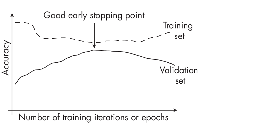
In Figure 1.1, we can see that the validation accuracy increases as the training and validation accuracy gap closes. The point where the training and validation accuracy is closest is the point with the least amount of overfitting, which is usually a good point for early stopping.

Smaller Models

Classic bias-variance theory suggests that reducing model size can reduce overfitting. The intuition behind this theory is that, as a general rule of thumb, the smaller the number of model parameters, the smaller its capacity to memorize or overfit to noise in the data. The following paragraphs discuss methods to reduce the model size, including pruning, which removes parameters from a model, and knowledge distillation, which transfers knowledge to a smaller model.

Besides reducing the number of layers and shrinking the layers’ widths as a hyperparameter tuning procedure, another approach to obtaining smal-  ler models is iterative pruning, in which we train a large model to achieve good performance on the original dataset. We then iteratively remove parameters of the model, retraining it on the dataset such that it maintains the same predictive performance as the original model. (The lottery ticket hypothesis, discussed in Chapter [ch04], uses iterative pruning.)

Another common approach to obtaining smaller models is knowledge distillation. The general idea behind this approach is to transfer knowledge from a large, more complex model (the teacher) to a smaller model (the student). Ideally, the student achieves the same predictive accuracy as the teacher, but it does so more efficiently due to the smaller size. As a nice side effect, the smaller student may overfit less than the larger teacher model. Figure [fig:ch06-fig02] diagrams the original knowledge distillation process. Here, the teacher is first trained in a regular supervised fashion to classify the examples in the dataset well, using a conventional cross-entropy loss between the predicted scores and ground truth class labels. While the smaller student network is trained on the same dataset, the training objective is to minimize both (a) the cross entropy between the outputs and the class labels and (b) the difference between its outputs and the teacher outputs (measured using Kullback–Leibler divergence, which quantifies the difference between two probability distributions by calculating how much one distribution diverges from the other in terms of information content).

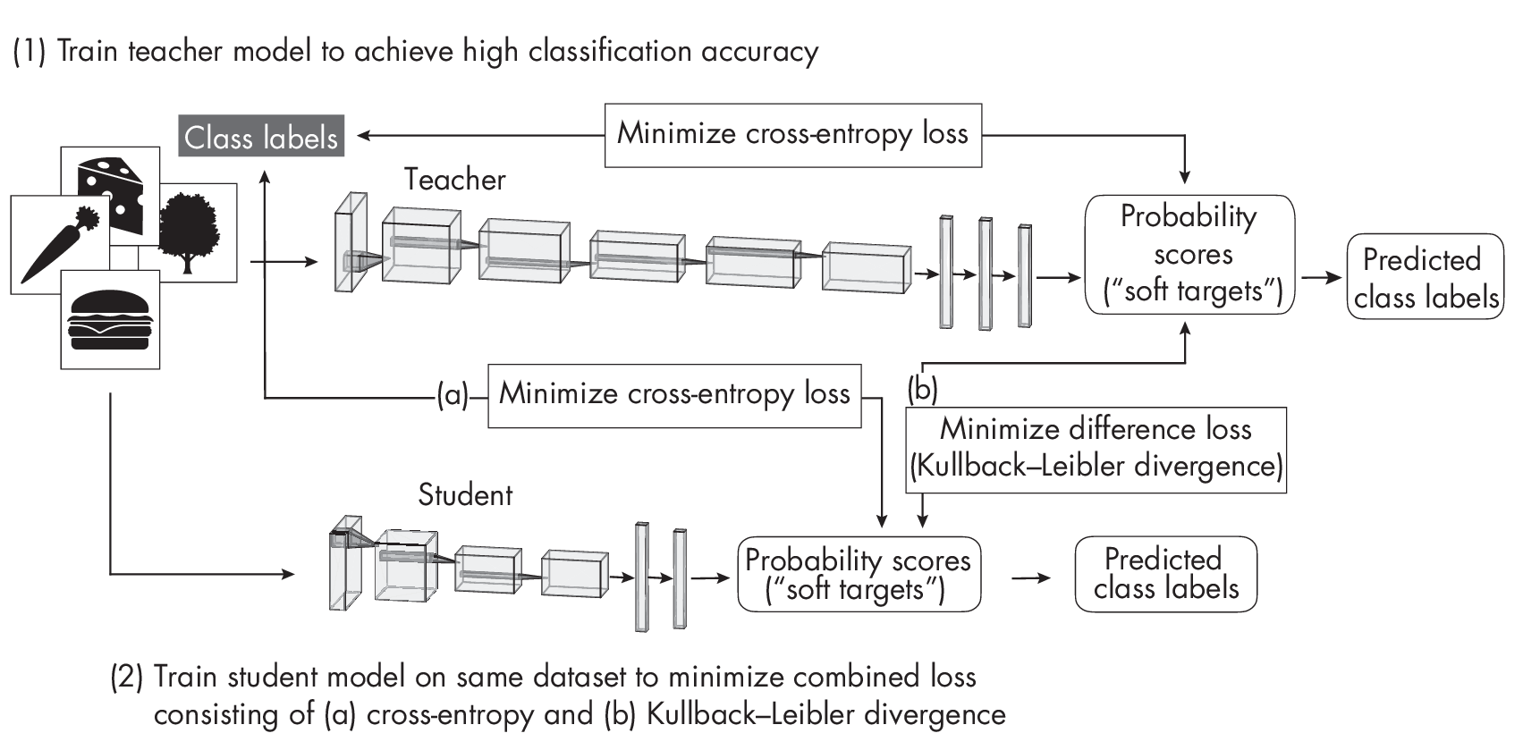
By minimizing the Kullback–Leibler divergence—the difference between the teacher and student score distributions—the student learns to mimic the teacher while being smaller and more efficient.

Caveats with Smaller Models

While pruning and knowledge distillation can also enhance a model’s generalization performance, these techniques are not primary or effective ways of reducing overfitting.

Early research results indicate that pruning and knowledge distillation can improve the generalization performance, presumably due to smaller model sizes. However, counterintuitively, recent research studying phenomena like double descent and grokking also showed that larger, overparameterized models have improved generalization performance if they are trained beyond the point of overfitting. Double descent refers to the phenomenon in which models with either a small or an extremely large number of para-  meters have good generalization performance, while models with a number of parameters equal to the number of training data points have poor generalization performance. Grokking reveals that as the size of a dataset decreases, the need for optimization increases, and generalization performance can improve well past the point of overfitting.

How can we reconcile the observation that pruned models can exhibit better generalization performance with contradictory observations from studies of double descent and grokking? Researchers recently showed that the improved training process partly explains the reduction of overfitting due to pruning. Pruning involves more extended training periods and a replay of learning rate schedules that may be partly responsible for the improved generalization performance.

Pruning and knowledge distillation remain excellent ways to improve the computational efficiency of a model. However, while they can also enhance a model’s generalization performance, these techniques are not primary or effective ways of reducing overfitting.

Ensemble Methods

Ensemble methods combine predictions from multiple models to improve the overall prediction performance. However, the downside of using multiple models is an increased computational cost.

We can think of ensemble methods as asking a committee of experts to weigh in on a decision and then combining their judgments in some way to make a final decision. Members in a committee often have different backgrounds and experiences. While they tend to agree on basic decisions, they can overrule bad decisions by majority rule. This doesn’t mean that the majority of experts is always right, but there is a good chance that the majority of the committee is more often right, on average, than every single member.

The most basic example of an ensemble method is majority voting. Here, we train k different classifiers and collect the predicted class label from each of these k models for a given input. We then return the most frequent class label as the final prediction. (Ties are usually resolved using a confidence score, randomly picking a label, or picking the class label with the lowest index.)

Ensemble methods are more prevalent in classical machine learning than deep learning because it is more computationally expensive to employ multiple models than to rely on a single one. In other words, deep neural networks require significant computational resources, making them less suitable for ensemble methods.

Random forests and gradient boosting are popular examples of ensemble methods. However, by using majority voting or stacking, for example, we can combine any group of models: an ensemble may consist of a support vector machine, a multilayer perceptron, and a nearest-neighbor classifier. Here, stacking (also known as stacked generalization)is a more advanced variant of majority voting that involves training a new model to combine the predictions of several other models rather than obtaining the label by majorit yvote.

A popular industry technique is to build models from k-fold cross-validation, a model evaluationt echnique in which we train and evaluate a model on k training folds.We then compute the average performance metric across all k iterations to estimate the overall performance measure of the model. After evaluation, we can either train the model on the entire training dataset or combine the individual models as an ensemble, as shown in Figure 1.2.

k-fold cross-validation for creating model ensembles

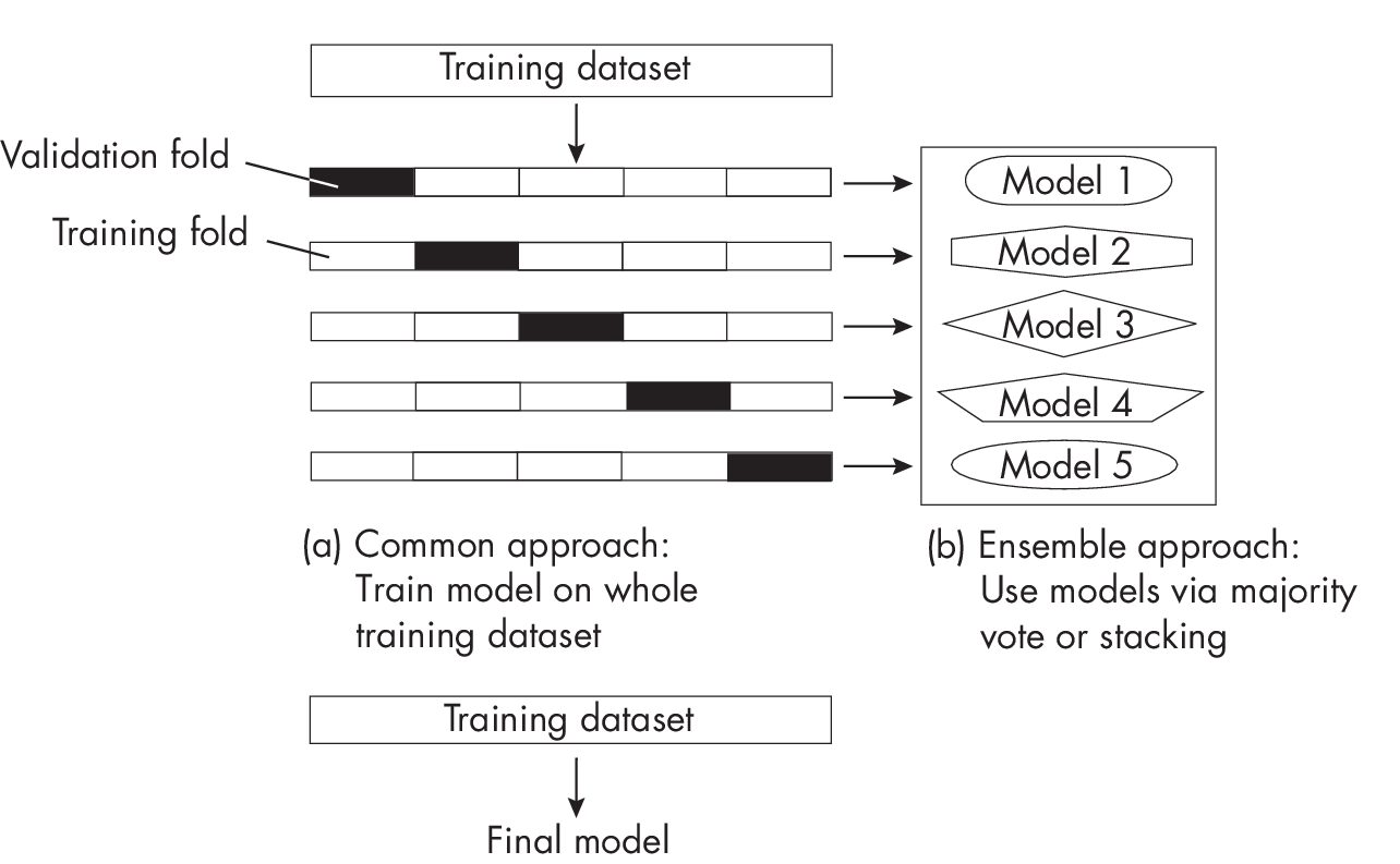
As shown in Figure 1.2, the k-fold ensemble approach trains each of the k models on the respective k – 1 training folds in each round. After evaluating the models on the validation folds, we can combine them into a majority vote classifier or build an ensemble using stacking, a technique that combines multiple classification or regression models via a meta-model.

While the ensemble approach can potentially reduce overfitting and improve robustness, this approach is not always suitable. For instance, potential downsides include managing and deploying an ensemble of models, which can be more complex and computationally expensive than using a single model.

Other Methods

So far, this book has covered some of the most prominent techniques to reduce overfitting. Chapter [ch05] covered techniques that aim to reduce overfitting from a data perspective. Additional techniques for reducing overfitting with model modifications include skip-connections (found in residual networks, for example), look-ahead optimizers, stochastic weight averaging, multitask learning, and snapshot ensembles.

While they are not originally designed to reduce overfitting, layer input normalization techniques such as batch normalization (BatchNorm) and layer normalization (LayerNorm) can stabilize training and often have a regularizing effect that reduces overfitting. Weight normalization, which normalizes the model weights instead of layer inputs, could also lead to better generalization performance. However, this effect is less direct since weight normalization (WeightNorm) doesn’t explicitly act as a regularizer like weight decay does.

Choosing a Regularization Technique

Improving data quality is an essential first step in reducing overfitting. However, for recent deep neural networks with large numbers of parameters, we need to do more to achieve an acceptable level of overfitting. Therefore, data augmentation and pretraining, along with established techniques such as dropout and weight decay, remain crucial overfitting reduction methods.

In practice, we can and should use multiple methods at once to reduce overfitting for an additive effect. To achieve the best results, treat selecting these techniques as a hyperparameter optimization problem.

Exercises

6-1. Supposewe’reusingearlystoppingasamechanismtoreduceover-  fitting—inparticular,amodernearly-stoppingvariantthatcreates checkpoints of the best model (for instance, the model with the high-  est validation accuracy) during training so that we can load it after the training has completed. This mechanism can be enabled in most modern deep learning frameworks. However, a colleague recommends tuning the number of training epochs instead. What are some of the advantages and disadvantages of each approach?

6-2. Ensemble models have been established as a reliable and successful method for decreasing overfitting and enhancing the reliability of predictive modeling efforts. However, there’s always a trade-off. What are some of the drawbacks associated with ensemble techniques?

References

• For more on the distinction between L₂ regularization and weight decay: Guodong Zhang et al., “Three Mechanisms of Weight Decay Regularization” (2018), https://arxiv.org/abs/1810.12281.

• Research results indicate that pruning and knowledge distillation can improve generalization performance, presumably due to smaller model sizes: Geoffrey Hinton, Oriol Vinyals, and Jeff Dean, “Distilling the Knowledge in a Neural Network” (2015), https://arxiv.org/abs/1503.02531.

• Classic bias-variance theory suggests that reducing model size can reduce overfitting: Jerome H. Friedman, Robert Tibshirani, and Trevor Hastie, “Model Selection and Bias-Variance Tradeoff,” Chapter 2.9, in The Elements of Statistical Learning (Springer, 2009).

• The lottery ticket hypothesis applies knowledge distillation to find smaller networks with the same predictive performance as the original one: Jonathan Frankle and Michael Carbin, “The Lottery Ticket Hypothesis: Finding Sparse, Trainable Neural Networks” (2018), https://arxiv.org/abs/1803.03635.

• For more on double descent: https://en.wikipedia.org/wiki/Double_descent.

• The phenomenon of grokking indicates that generalization perfor-  mance can improve well past the point of overfitting: Alethea Power et al., “Grokking: Generalization Beyond Overfitting on Small Algorithmic Datasets” (2022), https://arxiv.org/abs/2201.02177.

• Recent research shows that the improved training process partly explains the reduction of overfitting due to pruning: Tian Jin et al., “Pruning’s Effect on Generalization Through the Lens of Training and Regularization” (2022), https://arxiv.org/abs/2210.13738.

• Dropout was previously discussed as a regularization technique, but it can also be considered an ensemble method that approximates a weighted geometric mean of multiple networks: Pierre Baldi and Peter J. Sadowski, “Understanding Dropout” (2013), https://proceedings.neurips.cc/paper/2013/hash/71f6278d140af599 e06ad9bf1ba03cb0-Abstract.html.

• Regularization cocktails need to be tuned on a per-dataset basis: Arlind Kadra et al., “Well-Tuned Simple Nets Excel on Tabular Datasets” (2021), https://arxiv.org/abs/2106.11189.