Chapter 2: Self-Supervised Learning

What is self-supervised learning, when is it useful, and what are the main approaches to implementing it?

Self-supervised learning is a pretraining procedure that lets neural networks leverage large, unlabeled datasets in a supervised fashion. This chapter compares self-supervised learning to transfer learning, a related method for pretraining neural networks, and discusses the practical applications of self-supervised learning. Finally, it outlines the main categories of self-supervised learning.

Self-Supervised Learning vs. Transfer Learning

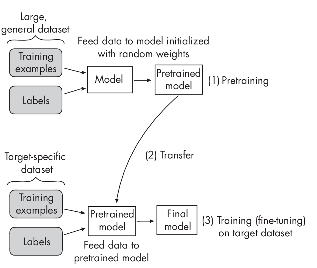
Self-supervised learning is related to transfer learning, a technique in which a model pretrained on one task is reused as the starting point for a model on a second task. For example, suppose we are interested in training an image classifier to classify bird species. In transfer learning, we would pretrain a convolutional neural network on the ImageNet dataset, a large, labeled image dataset with many different categories, including various objects and animals. After pretraining on the general ImageNet dataset, we would take that pretrained model and train it on the smaller, more specific target dataset that contains the bird species of interest. (Often, we just have to change the class-specific output layer, but we can otherwise adopt the pretrained network as is.)

Figure 1.1 illustrates the process of transfer learning.

Pretraining with conventional transfer learning

Self-supervised learning is an alternative approach to transfer learning in which the model is pretrained not on labeled data but on unlabeled data. We consider an unlabeled dataset for which we do not have label information, and then we find a way to obtain labels from the dataset’s structure to formulate a prediction task for the neural network, as illustrated in Figure 1.2. These self-supervised training tasks are also called pretext tasks.

Pretraining with self-supervised learning

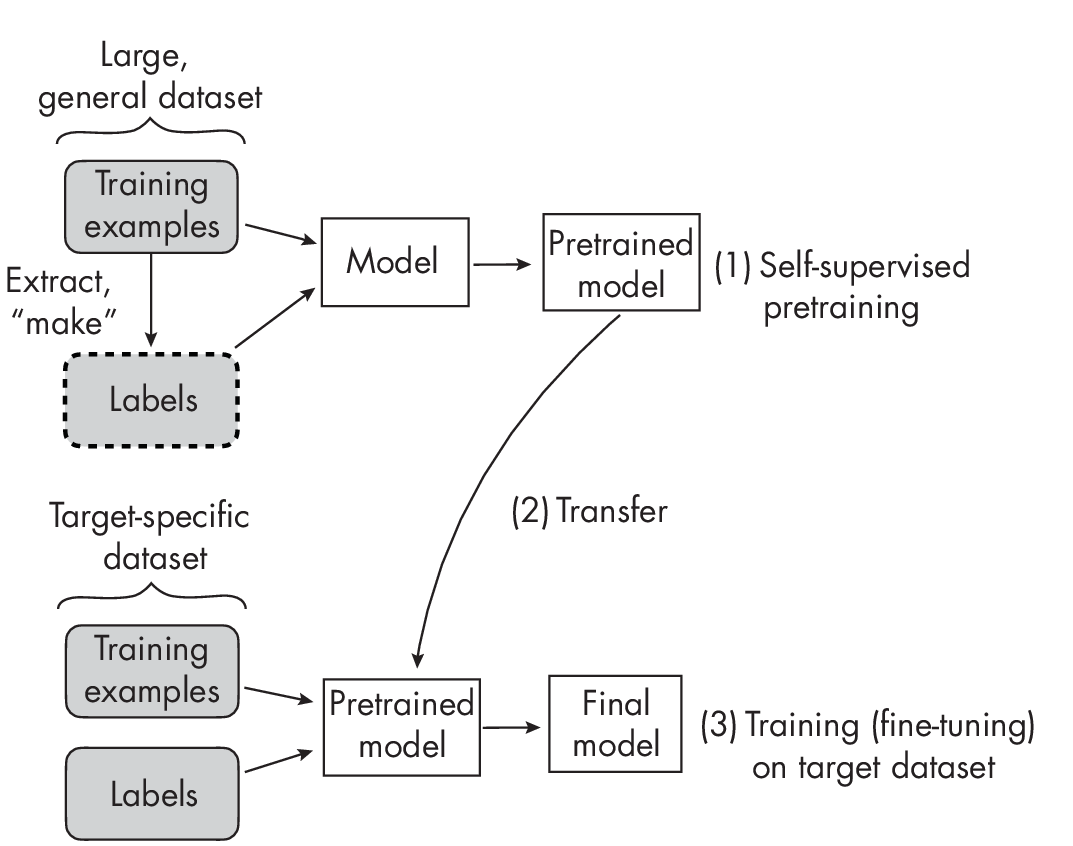
The main difference between transfer learning and self-supervised learning lies in how we obtain the labels during step 1 in Figures 1.1 and 1.2. In transfer learning, we assume that the labels are provided along with the data-  set; they are typically created by human labelers. In self-supervised learning, the labels can be directly derived from the training examples.

A self-supervised learning task could be a missing-word prediction in a natural language processing context. For example, given the sentence “It is beautiful and sunny outside,” we can mask out the word sunny, feed the network the input “It is beautiful and [MASK] outside,” and have the network predict the missing word in the “[MASK]” location. Similarly, we could remove image patches in a computer vision context and have the neural network fill in the blanks. These are just two examples of self-supervised learning tasks; many more methods and paradigms for this type of learning exist.

In sum, we can think of self-supervised learning on the pretext task as representation learning. We can take the pretrained model to fine-tune it on the target task (also known as the downstream task).

Leveraging Unlabeled Data

Large neural network architectures require large amounts of labeled data to perform and generalize well. However, for many problem areas, we don’t have access to large labeled datasets. With self-supervised learning, we can leverage unlabeled data. Hence, self-supervised learning is likely to be useful when working with large neural networks and with a limited quantity of labeled training data.

Transformer-based architectures that form the basis of LLMs and vision transformers are known to require self-supervised learning for pretraining to perform well.

For small neural network models such as multilayer perceptrons with two or three layers, self-supervised learning is typically considered neither useful nor necessary.

Self-supervised learning likewise isn’t useful in traditional machine learning with nonparametric models such as tree-based random forests or gradient boosting. Conventional tree-based methods do not have a fixed parameter structure (in contrast to the weight matrices, for example). Thus, conventional tree-based methods are not capable of transfer learning and are incompatible with self-supervised learning.

Self-Prediction and Contrastive Self-Supervised Learning

There are two main categories of self-supervised learning: self-prediction and contrastive self-supervised learning. In self-prediction, illustrated in Figure 1.3, we typically change or hide parts of the input and train the mo-  del to reconstruct the original inputs, such as by using a perturbation mask that obfuscates certain pixels in an image.

Self-prediction after applying a
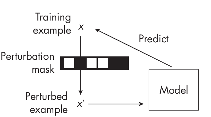
perturbation mask

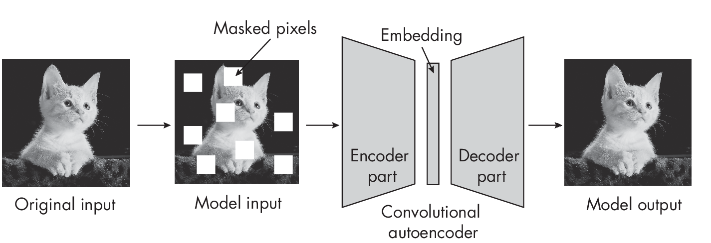
A classic example is a denoising autoencoder that learns to remove noise from an input image. Alternatively, consider a masked autoencoder that reconstructs the missing parts of an image, as shown in Figure 1.4.

A masked autoencoder reconstructing a masked image

Missing (masked) input self-prediction methods are also commonly used in natural language processing contexts. Many generative LLMs, such as GPT, are trained on a next-word prediction pretext task (GPT will be discussed at greater length in Chapters [ch14] and [ch17]). Here, we feed the network text fragments, where it has to predict the next word in the sequence (as we’ll discuss further in Chapter [ch17]).

In contrastive self-supervised learning, we train the neural network to learn an embedding space where similar inputs are close to each other and dissimilar inputs are far apart. In other words, we train the network to produce embeddings that minimize the distance between similar training inputs and maximize the distance between dissimilar training examples.

Let’s discuss contrastive learning using concrete example inputs. Suppose we have a dataset consisting of random animal images. First, we draw a random image of a cat (the network does not know the label, because we assume that the dataset is unlabeled). We then augment, corrupt, or perturb this cat image, such as by adding a random noise layer and cropping it differently, as shown in Figure 1.5.

Image pairs encountered in contrastive learning

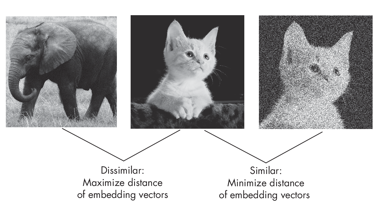
The perturbed cat image in this figure still shows the same cat, so we want the network to produce a similar embedding vector. We also consider a random image drawn from the training set (for example, an elephant, but again, the network doesn’t know the label).

For the cat-elephant pair, we want the network to produce dissimilar embeddings. This way, we implicitly force the network to capture the image’s core content while being somewhat agnostic to small differences and noise. For example, the simplest form of a contrastive loss is the L₂-norm (Euclidean distance) between the embeddings produced by model M(\(\cdot\)). Let’s say we update the model weights to decrease the distance \(||\)M(cat) – M(cat\('\))\(||\)₂ and increase the distance \(||\)M(cat) – M(elephant)\(||\)₂.

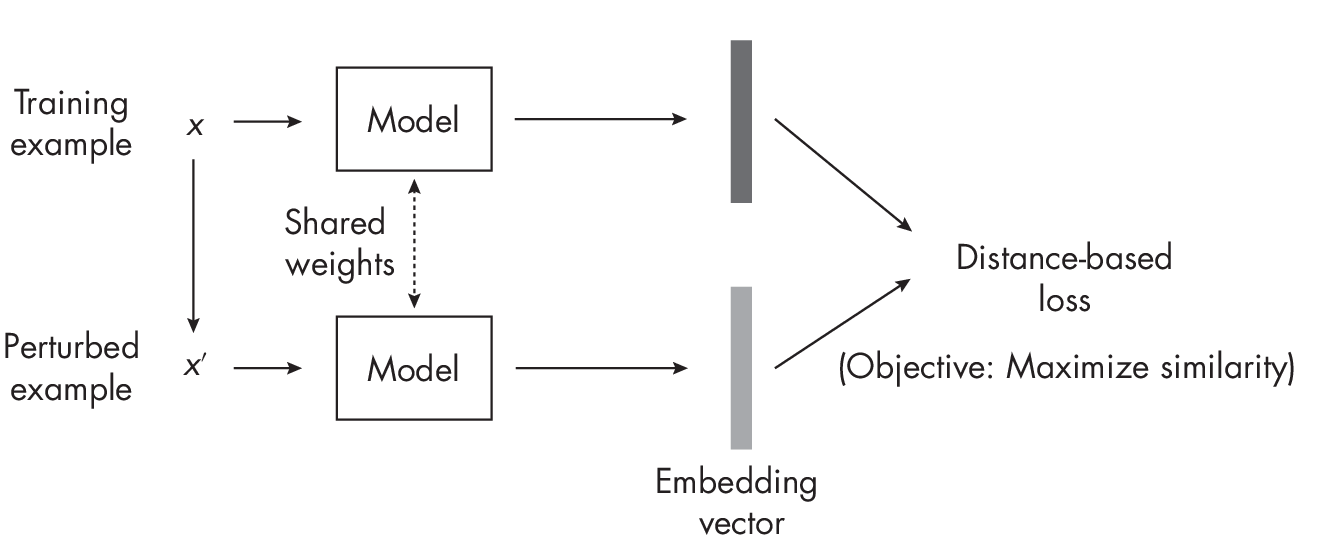
Figure 1.6 summarizes the central concept behind contrastive learning for the perturbed image scenario. The model is shown twice, which is known as a siamese network setup. Essentially, the same model is utilized in two instances: first, to generate the embedding for the original training example, and second, to produce the embedding for the perturbed version of the sample.

Contrastive learning

This example outlines the main idea behind contrastive learning, but many subvariants exist. Broadly, we can categorize these into sample contrastive and dimension contrastive methods. The elephant-cat example in Figure 1.6 illustrates a sample contrastive method, where we focus on learning embeddings to minimize and maximize distances between training pairs. In dimension-contrastive approaches, on the other hand, we focus on making only certain variables in the embedding representations of similar training pairs appear close to each other while maximizing the distance of others.

Exercises

2-1. How could we apply self-supervised learning to video data?

2-2. Can self-supervised learning be used for tabular data represented as rows and columns? If so, how could we approach this?

References

• For more on the ImageNet dataset: https://en.wikipedia.org/wiki/ImageNet.

• An example of a contrastive self-supervised learning method: Ting Chen et al., “A Simple Framework for Contrastive Learning of Visual Representations” (2020), https://arxiv.org/abs/2002.05709.

• An example of a dimension-contrastive method: Adrien Bardes, Jean Ponce, and Yann LeCun, “VICRegL: Self-Supervised Learning of Local Visual Features” (2022), https://arxiv.org/abs/2210.01571.

• If you plan to employ self-supervised learning in practice: Randall Balestriero et al., “A Cookbook of Self-Supervised Learning” (2023), https://arxiv.org/abs/2304.12210.

• A paper proposing a method of transfer learning and self-supervised learning for relatively small multilayer perceptrons on tabular datasets: Dara Bahri et al., “SCARF: Self-Supervised Contrastive Learning Using Random Feature Corruption” (2021), https://arxiv.org/abs/2106.15147.

• A second paper proposing such a method: Roman Levin et al., “Transfer Learning with Deep Tabular Models” (2022), https://arxiv.org/abs/ 2206.15306.