Creating Confidence Intervals for Machine Learning Classifiers
Developing good predictive models hinges upon accurate performance evaluation and comparisons. However, when evaluating machine learning models, we typically have to work around many constraints, including limited data, independence violations, and sampling biases. Confidence intervals are no silver bullet, but at the very least, they can offer an additional glimpse into the uncertainty of the reported accuracy and performance of a model.
As Steinbach et al. recently noted,
confidence intervals around accuracy measurements can greatly enhance the communication of research results as well as impact the reviewing process.
In my experience as a reviewer, I have seen many research articles that adopted this suggested minimal standard by including uncertainty estimates. However, many articles still omit any form of uncertainty estimates, and, moving forward, I hope we can increase the adoption as it is usually just a small thing to add.
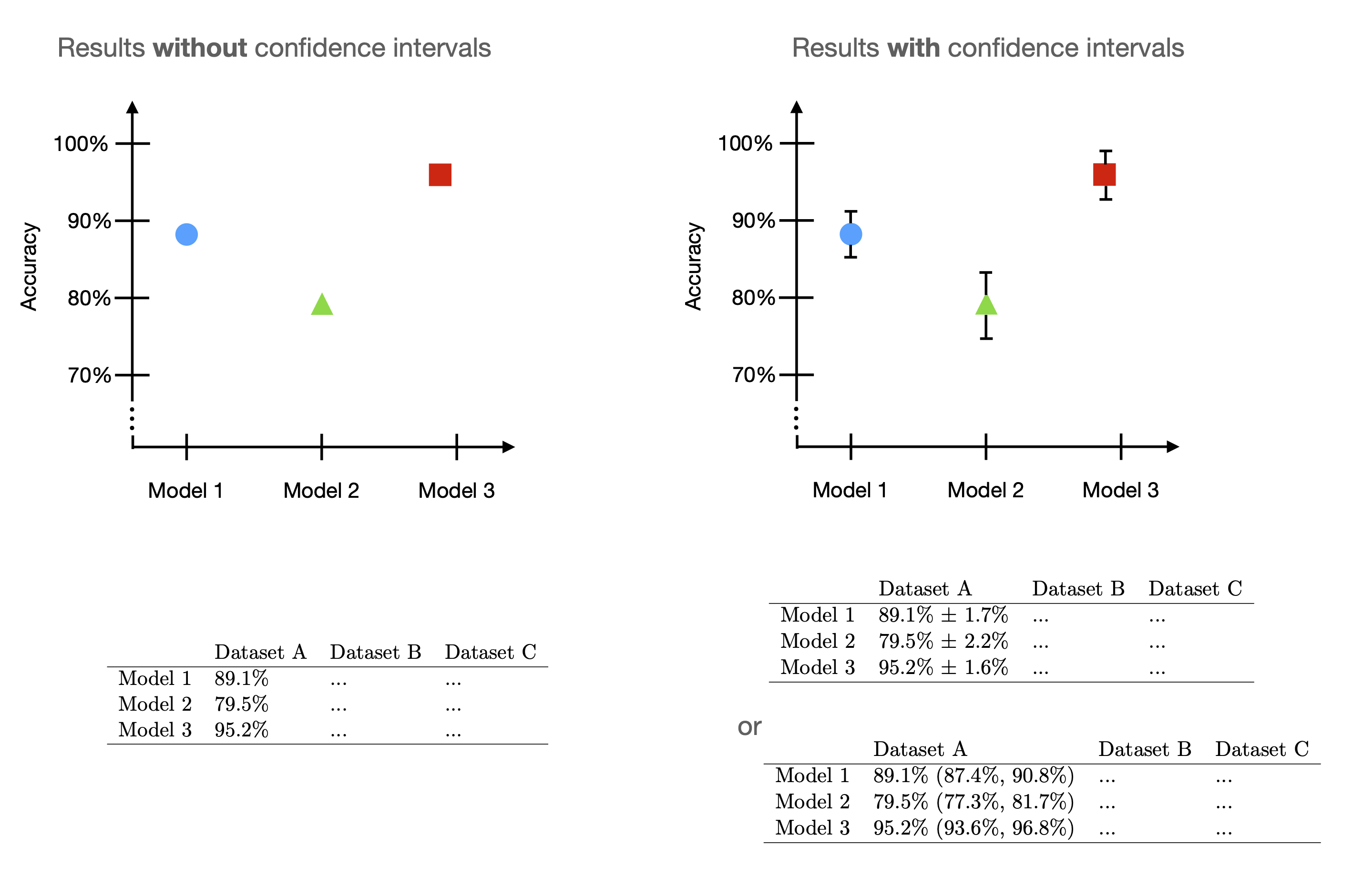
This article outlines different methods for creating confidence intervals for machine learning models. Note that these methods also apply to deep learning. This article is purposefully short to focus on the technical execution without getting bogged down in details; there are many links to all the relevant conceptual explanations throughout this article.
Lastly, it’s worth highlighting that the big picture is to measure and report uncertainty. Confidence intervals are one way to do that. However, It is also helpful to include the average performance over different dataset splits or random seeds with the variance or standard deviation – I sometimes adopt this simpler approach as it is more straightforward to explain. But since this article is about confidence intervals, let’s define what they are and how we can construct them.
Confidence Intervals in a Nutshell
In a nutshell, what is a confidence interval anyway? A confidence interval is a method that computes an upper and a lower bound around an estimated value. The actual parameter value is either insider or outside these bounds.
Imagine that we have a statistic like a sample mean that we calculated from a sample drawn from an unknown population. Our goal is to estimate a population parameter with this statistic; for example, we could estimate the population mean using the sample mean. However, most of the time, the estimated and actual values are not exactly the same. Here, we can use the confidence interval to quantify the uncertainty of that estimate.
It is a common convention to use a 95% confidence interval in practice, but how do we interpret it? First, let’s assume we have access to the population. (This is, of course, never the case. Otherwise, we wouldn’t have to estimate a parameter but could compute it precisely.) Then, if we draw a very large number of samples from the distribution and apply our confidence interval method to these samples, 95% of the confidence intervals would contain the actual value.

In a machine learning context, what we are usually interested in is the performance of our model. So, here the population parameter we want to estimate could be the generalization accuracy of our model. Then, the test set accuracy represents our estimated generalization accuracy. Finally, the 95% confidence interval gives us an uncertainty measure of how accurate this estimate is.
A Note About Statistical Significance
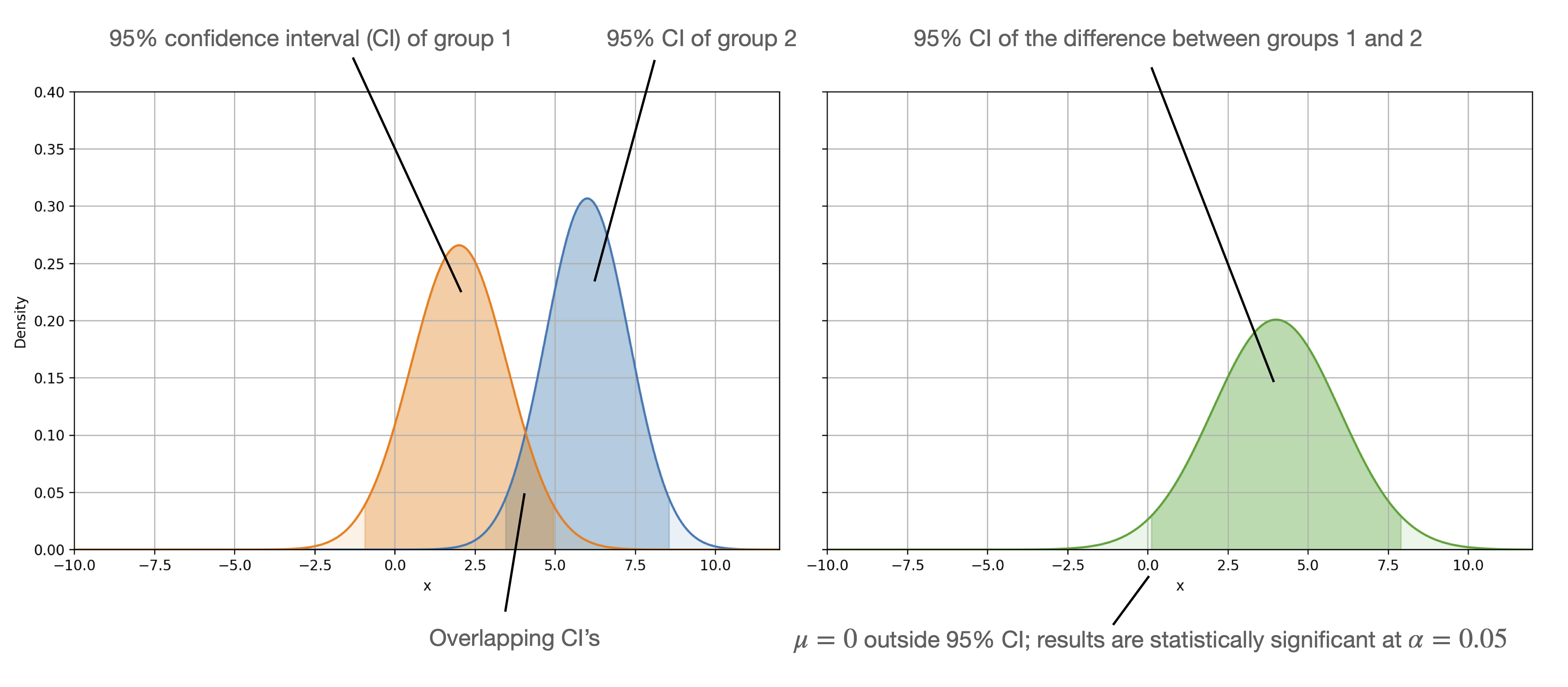
As a side-note, we can say that the difference of two measurements is statistically significant if confidence intervals do not overlap. However we cannot say that results are not statistically significant if confidence intervals overlap. (The Error bars article in the Points of Significance series illustrates this nicely.) If we want to check whether the difference is not statistical significant, we would have to take a look at the distribution of the differences we want to compare and check whether its confidence interval contains 0 or not.
Defining a Dataset and Model for Hands-On Examples
The following sections will show some common ways of constructing confidence intervals for machine learning classifier performances.
We will use the Iris dataset and a decision tree classifier for simplicity. However, these methods generalize to other datasets and classifiers, including deep neural networks.
(A Jupyter notebook containing the code examples can be found here.)
In:
from mlxtend.data import iris_data
from sklearn.model_selection import train_test_split
from sklearn.tree import DecisionTreeClassifier

X, y = iris_data()

X_train, X_test, y_train, y_test = train_test_split(
    X, y, test_size=0.15, random_state=123, stratify=y
)

clf = DecisionTreeClassifier(random_state=123)
Method 1: Normal Approximation Interval Based on a Test Set
The normal approximation interval is maybe the easiest and most classic way of creating confidence intervals. Using this method, we compute the confidence interval from a single training-test split. This is particularly attractive in deep learning where model training is expensive. It’s also attractive (usually in a deep learning context) when we are interested in a very particular model (vs. models fit on different training folds like in k-fold cross-validation).
In a nutshell, the equation for computing the confidence interval for an estimated parameter (let’s say the the sample mean \(\bar{x}\)) assuming a normal distribution is computed as follows: \(\bar{x} \pm z \times \text{SE},\)
where
- \(z\) is the \(z\) value (the number of standard deviations that a value lies from the mean of a standard normal distribution);
- \(\text{SE}\) is the standard error of the estimated parameter (here: sample mean).
In our case, the sample mean \(\bar{x}\) is test set accuracy \(\text{ACC}_{\text{test}}\), a proportion of success (in the context of a Binomial proportion confidence interval).
The standard error, under a normal approximation can be computed as
\[\text{SE} = \sqrt{ \frac{1}{n} \text{ACC}_{\text{test}}\left(1- \text{ACC}_{\text{test}}\right)},\]where \(n\) is the test set size. So, plugging the SE back into the formula above, we get
\[\text{ACC}_{\text{test}} \pm z \sqrt{\frac{1}{n} \text{ACC}_{\text{test}}\left(1- \text{ACC}_{\text{test}}\right)}.\](You can find a description of this method in section 1.7 Confidence Intervals via Normal Approximation of my “Model Evaluation, Model Selection, and Algorithm Selection in Machine Learning”.)
Now, let’s see how we can code this in Pyhon. We start with computing the z-value, which can obtain from scipy.stats.norm.ppf (rather than looking it up from a \(z\) table in one of our old statistics textbooks).
In:
import scipy.stats

confidence = 0.95  # Change to your desired confidence level
z_value = scipy.stats.norm.ppf((1 + confidence) / 2.0)
print(z_value)
Out:
1.959963984540054
Next, let’s compute the test accuracy of the classifier and plug the values into the formula above; the Python code for this is as follows:
In:
import numpy as np

clf.fit(X_train, y_train)

acc_test = clf.score(X_test, y_test)
ci_length = z_value * np.sqrt((acc_test * (1 - acc_test)) / y_test.shape[0])

ci_lower = acc_test - ci_length
ci_upper = acc_test + ci_length

print(ci_lower, ci_upper)
Out:
0.873179017733963 1.0398644605269067
So, the above values represent the 95% confidence interval around the test set accuracy. Let’s visualize the confidence interval using the following code:
In:
import matplotlib.pyplot as plt

fig, ax = plt.subplots(figsize=(7, 3))

ax.errorbar(acc_test, 0, xerr=ci_length, fmt="o")

ax.set_xlim([0.8, 1.0])

ax.set_yticks(np.arange(1))
ax.set_yticklabels(["Normal approximation interval"])
ax.set_xlabel("Prediction accuracy")

plt.tight_layout()
plt.grid(axis="x")
plt.show()
Out:
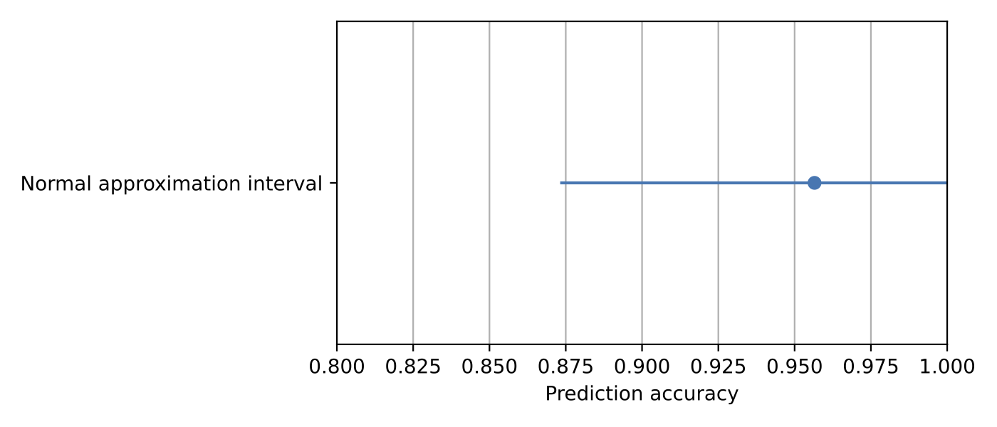
We cut the upper confidence interval bound at 1.0 (the 100% accuracy mark) since reporting an accuracy value exceeding 100% doesn’t make sense.
Lastly, let’s store our confidence interval in a Python dictionary so that we can retrieve it later when we compare it to other confidence intervals:
In:
results = {
    "Method 1: Normal approximation": {
        "Test accuracy": acc_test,
        "Lower 95% CI": ci_lower,
        "Upper 95% CI": ci_upper,
    }
}
Method 2: Bootstrapping Training Sets – Setup Step
Confidence intervals are used to estimate unknown parameters. If we only have one estimate, like the accuracy from a single test set, we need to make assumptions about the distribution of this accuracy value. For example, we may assume that the accuracy values (that we would compute from different samples) are normally distributed.
In an ideal world, we have access to our test set sample’s distribution. If that’s the case, we could look at the range of values that 95% of the accuracy values fall into. This is desirable but not practical since we don’t have an infinite pool of test sets. Now, a workaround is bootstrapping, which estimates the sampling distribution. This is done by taking multiple samples with replacement from a single random sample. The equation is as follows: \(\text{ACC}_{\text{bootavg}}=\frac{1}{b} \sum_{j=1}^{b} \text{ACC}_{\text{boot}, j},\)
where \(b\) is the number of bootstrap rounds, and \(\text{ACC}_{\text{boot}, j}\) is the model accuracy computed in the \(j\)-th round. Note that 200 is usually recommended as the minimum number of bootstrap rounds (see “Introduction to the Bootstrap” book).
The method we use for evaluating machine learning models is often referred to as out-of-bag bootstrap. We train the model on training folds and assess it on held-out data points from each round. For more detail, please see section 2, Bootstrapping and Uncertainties of “Model Evaluation, Model Selection, and Algorithm Selection in Machine Learning.” However, there are different flavors of bootstrapping. Below, we create multiple bootstrap samples for re-use in the upcoming sections.
In:
import numpy as np

rng = np.random.RandomState(seed=12345)
idx = np.arange(y_train.shape[0])

bootstrap_train_accuracies = []
bootstrap_rounds = 200


for i in range(bootstrap_rounds):

    train_idx = rng.choice(idx, size=idx.shape[0], replace=True)
    valid_idx = np.setdiff1d(idx, train_idx, assume_unique=False)

    boot_train_X, boot_train_y = X_train[train_idx], y_train[train_idx]
    boot_valid_X, boot_valid_y = X_train[valid_idx], y_train[valid_idx]

    clf.fit(boot_train_X, boot_train_y)
    acc = clf.score(boot_valid_X, boot_valid_y)
    bootstrap_train_accuracies.append(acc)

bootstrap_train_mean = np.mean(bootstrap_train_accuracies)
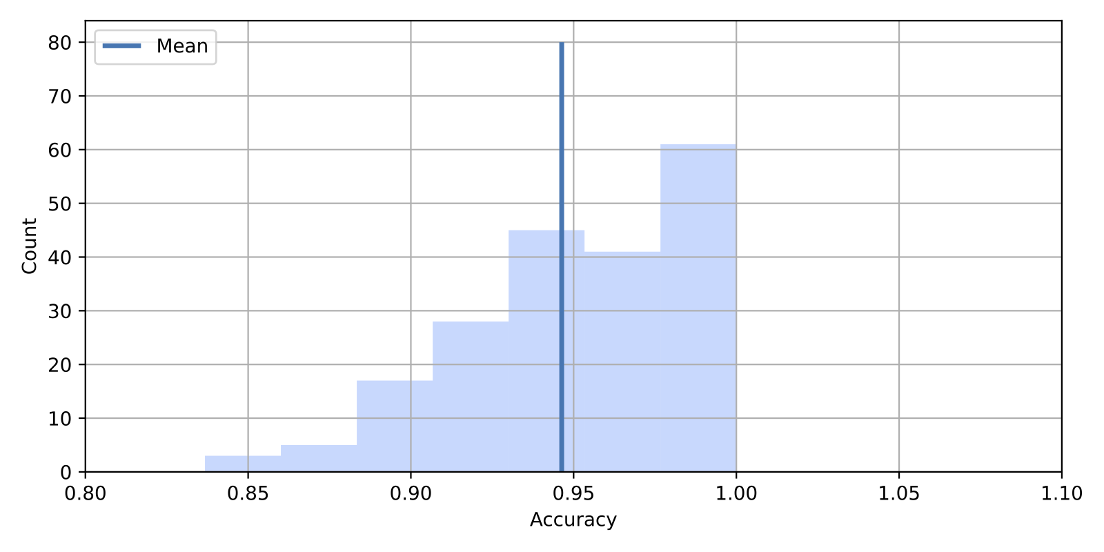
We can visualize the test accuracies from bootstrapping (\(\text{ACC}_{\text{boot}, j}\)) along with their sample mean (\(\text{ACC}_{\text{bootavg}}\)) in a historgram via the code below:
In:
fig, ax = plt.subplots(figsize=(8, 4))

ax.vlines(bootstrap_train_mean, [0], 80, lw=2.5, linestyle="-", label="Mean")

ax.hist(
    bootstrap_train_accuracies, bins=7, color="#0080ff", edgecolor="none", alpha=0.3
)

plt.xlabel('Accuracy')
plt.ylabel('Count')
plt.xlim([0.8, 1.1])

plt.legend(loc="upper left")
plt.grid()
plt.show()
A Note About Replacing Independent Test Sets with Bootstrapping
We created validation (or test) sets from the training set via bootstrapping in the section above. However, suppose we don’t tune our model on the training set. In that case, we can use the whole dataset and report the averaged bootstrap accuracy \(\text{ACC}_{\text{bootavg}}\) as your model performance estimate instead of using an independent test set. This is particularly attractive for small datasets. Moreover, as Bouthillier et al. found in their Accounting for variance in machine learning benchmarks study, using an out-of-bag bootstrap procedure can improve the reliability of the performance estimation.
Method 2.1: A t Confidence Interval from Bootstrap Samples
Now that we introduced the out-of-bag bootstrapping procedure let’s get to the interesting part and compute the confidence interval from the bootstrap samples. Assuming that the sample means are normal distributed we could compute the confidence interval formula as before, as follows:
\[\text{ACC}_{\text{test}} \pm z \times \text{SE}.\]Generally, it is common to replace the \(z\) value with a \(t\) value if we deal with finite sample sizes and want to estimate the population standard deviation via the sample standard deviation (the standard deviation is used to calculate the standard error):
\[\text{ACC}_{\text{test}} \pm t \times \text{SE}.\]However, using \(z\) scores is absolutely fine because, for sample sizes larger than 100, the \(z\) and \(t\) scores are practically identical (here, we assume we have at least 200 bootstrap samples.)
We can then compute the standard error (SE) by the as the standard deviation of this distribution:
\[\text{SE}=\sqrt{\frac{1}{b-1} \sum_{j=1}^{b}\left(\text{ACC}_{\text{boot},j}-{\text{ACC}_\text{bootavg}}\right)^{2}}.\]Note that we usually divide the standard deviation (SD) by \(\sqrt{n}\) to obtain the standard error (SE) where \(n = b\):
\[\text{SE} = \frac{\text{SD}}{\sqrt{n}}.\]However, this is not necessary here since the bootstrap distribution is a distribution of means (as opposed to single data points), and \(\text{ACC}_{\text{bootavg}}\) is the mean of these means.
(As an optional exercise, you can try to modify the code below to include the division by \(\sqrt{n}\) (where \(\sqrt{n} = \sqrt{b}\)), and you will probably find that this shrinks the confidence interval to an unrealistic degree, which also doesn’t match the percentile method results anymore that we will introduce shortly.)
After all this setup, let’s get to the coding part. Again, instead of using a \(t\)-table in our old statistics textbook, let’s use SciPy to obtain the \(t\) value for a 95% confidence interval and \(b-1\) degrees of freedom:
In:
confidence = 0.95  # Change to your desired confidence level
t_value = scipy.stats.t.ppf((1 + confidence) / 2.0, df=bootstrap_rounds - 1)
print(t_value)
Out:
1.971956544249395
Next, let’s compute the 95% confidence interval:
In:
se = 0.0
for acc in bootstrap_train_accuracies:
    se += (acc - bootstrap_train_mean) ** 2
se = np.sqrt((1.0 / (bootstrap_rounds - 1)) * se)

ci_length = t_value * se

ci_lower = bootstrap_train_mean - ci_length
ci_upper = bootstrap_train_mean + ci_length

print(ci_lower, ci_upper)
Out:
0.879470830164037 1.0132047668825668
And, to make the results more visual, let’s add the confidence interval to our histogram plot:
In:
fig, ax = plt.subplots(figsize=(8, 4))
ax.vlines(bootstrap_train_mean, [0], 80, lw=2.5, linestyle="-", label="Mean")

ax.vlines(ci_lower, [0], 15, lw=2.5, linestyle="dotted", label="95% CI", color="C2")
ax.vlines(ci_upper, [0], 15, lw=2.5, linestyle="dotted", color="C2")

ax.hist(
    bootstrap_train_accuracies, bins=7, color="#0080ff", edgecolor="none", alpha=0.3
)

plt.xlabel('Accuracy')
plt.ylabel('Count')
plt.xlim([0.8, 1.1])

plt.legend(loc="upper left")

plt.grid()
plt.show()
Out:
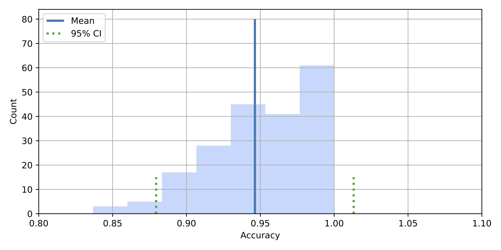
You might wonder how this compares to the normal approximation interval (Method 1) we created earlier? No worries, we will get to that in a later section.
Again, let’s add our CI values to the Python dictionary for a comparison study later.
In:
results["Method 2.1: Bootstrap, 1-sample CI"] = {
    "Test accuracy": bootstrap_train_mean,
    "Lower 95% CI": ci_lower,
    "Upper 95% CI": ci_upper,
}
Method 2.2: Bootstrap Confidence Intervals Using the Percentile Method
The approach outlined in the previous section seems pretty straightforward if our bootstrapped accuracies follow a normal distribution. However, a more robust and general approach for utilizing the bootstrap samples is the percentile method (see section 2, Bootstrapping and Uncertainties of my “Model Evaluation, Model Selection, and Algorithm Selection in Machine Learning” article for additional details).
Here, we pick our lower and upper confidence bounds as follows:
- \(\text{ACC}_{lower} = \alpha_{1}th\) percentile of the \(\text{ACC}_\text{boot}\) distribution;
- \(\text{ACC}_{upper} = \alpha_{2}th\) percentile of the \(\text{ACC}_{boot}\) distribution;
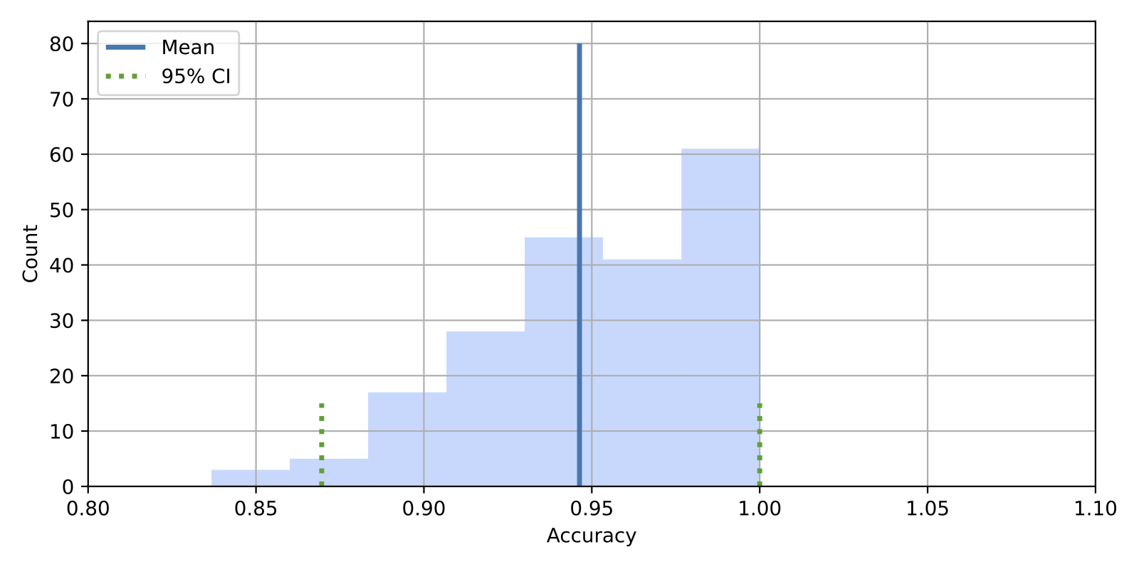
where \(\alpha_1 = \alpha\) and \(\alpha_2 = 1 - \alpha\), and \(\alpha\) is our degree of confidence to compute the \(100 \times (1 - 2 \times \alpha)\) confidence interval. For instance, to compute a 95% confidence interval, we pick \(\alpha = 0.025\) to obtain the 2.5th and 97.5th percentiles of the b bootstrap samples distribution as our upper and lower confidence bounds.
Using NumPy, computing the percentiles is pretty straightforward:
In:
ci_lower = np.percentile(bootstrap_train_accuracies, 2.5)
ci_upper = np.percentile(bootstrap_train_accuracies, 97.5)

print(ci_lower, ci_upper)
Out:
0.8695652173913043 1.0
As usual, let’s visualize the confidence interval in a histogram and update the results dictionary:
In:
fig, ax = plt.subplots(figsize=(8, 4))
ax.vlines(bootstrap_train_mean, [0], 80, lw=2.5, linestyle="-", label="Mean")

ax.vlines(ci_lower, [0], 15, lw=2.5, linestyle="dotted", label="95% CI", color="C2")
ax.vlines(ci_upper, [0], 15, lw=2.5, linestyle="dotted", color="C2")

ax.hist(
    bootstrap_train_accuracies, bins=7, color="#0080ff", edgecolor="none", alpha=0.3
)
plt.legend(loc="upper left")

plt.xlabel('Accuracy')
plt.ylabel('Count')
plt.xlim([0.8, 1.1])

plt.grid()
plt.show()
Out:
In:
results["Method 2.2: Bootstrap, percentile"] = {
    "Test accuracy": bootstrap_train_mean,
    "Lower 95% CI": ci_lower,
    "Upper 95% CI": ci_upper,
}
Method 2.3: Reweighting the Boostrap Samples via the .632 Bootstrap
In this section, we will take a look at the .632 Bootstrap, which builds on the previously introduced percentile method.
Skipping over the technical details, the previously introduced out-of-bag bootstrap method has a slight pessimistic bias, which means that it reports a test accuracy that is slightly worse than the true generalization accuracy of the model. The .632 bootstrap aims to correct this pessimitic bias. (To keep this article concise, please see section 2, Bootstrapping and Uncertainties of my “Model Evaluation, Model Selection, and Algorithm Selection in Machine Learning” article for a more detailed discussion).
We are skipping the formulas and jump directly into the code implementation (in practice, I recommend using my implementation in mlxtend). In a nutshell, you can think of it as a reweighted version of the bootstrap method we used earlier:
In:
rng = np.random.RandomState(seed=12345)
idx = np.arange(y_train.shape[0])

bootstrap_train_accuracies = []
bootstrap_rounds = 200
weight = 0.632

for i in range(bootstrap_rounds):

    train_idx = rng.choice(idx, size=idx.shape[0], replace=True)
    valid_idx = np.setdiff1d(idx, train_idx, assume_unique=False)

    boot_train_X, boot_train_y = X_train[train_idx], y_train[train_idx]
    boot_valid_X, boot_valid_y = X_train[valid_idx], y_train[valid_idx]

    clf.fit(boot_train_X, boot_train_y)
    valid_acc = clf.score(boot_valid_X, boot_valid_y)
    # predict training accuracy on the whole training set
    # as ib the original .632 boostrap paper
    # in Eq (6.12) in
    #    "Estimating the Error Rate of a Prediction Rule: Improvement
    #     on Cross-Validation"
    #     by B. Efron, 1983, https://doi.org/10.2307/2288636
    train_acc = clf.score(X_train, y_train)

    acc = weight * train_acc + (1.0 - weight) * valid_acc

    bootstrap_train_accuracies.append(acc)

bootstrap_train_mean = np.mean(bootstrap_train_accuracies)
bootstrap_train_mean
Out:
0.9677367193053941
In:
ci_lower = np.percentile(bootstrap_train_accuracies, 2.5)
ci_upper = np.percentile(bootstrap_train_accuracies, 97.5)

print(ci_lower, ci_upper)
Out:
0.9221417322834646 1.0
In:
results["Method 2.3: Bootstrap, .632"] = {
    "Test accuracy": bootstrap_train_mean,
    "Lower 95% CI": ci_lower,
    "Upper 95% CI": ci_upper,
}
Method 2.4: Taking the Reweighting One Step Further: The .632+ Bootstrap
The .632+ Bootstrap is an improvement over the .632 Bootstrap we implemented above. In a nutshell, the main difference is that the weighting terms are computed from the so-called no-information rate rather than being fixed.
Again, we are skipping the formulas, jumping directly into the code implementation. In practice, I recommend using my implementation in mlxtend. And for a more detailed discussion, please see section 2, Bootstrapping and Uncertainties of my “Model Evaluation, Model Selection, and Algorithm Selection in Machine Learning” article.
In:
from itertools import product

from sklearn.metrics import accuracy_score


def no_information_rate(targets, predictions, loss_fn):
    combinations = np.array(list(product(targets, predictions)))
    return loss_fn(combinations[:, 0], combinations[:, 1])


rng = np.random.RandomState(seed=12345)
idx = np.arange(y_train.shape[0])

bootstrap_train_accuracies = []
bootstrap_rounds = 200
weight = 0.632


for i in range(bootstrap_rounds):

    train_idx = rng.choice(idx, size=idx.shape[0], replace=True)
    valid_idx = np.setdiff1d(idx, train_idx, assume_unique=False)

    boot_train_X, boot_train_y = X_train[train_idx], y_train[train_idx]
    boot_valid_X, boot_valid_y = X_train[valid_idx], y_train[valid_idx]

    clf.fit(boot_train_X, boot_train_y)
    train_acc = clf.score(X_train, y_train)
    valid_acc = clf.score(boot_valid_X, boot_valid_y)

    gamma = no_information_rate(y, clf.predict(X), accuracy_score)
    R = (valid_acc - train_acc) / (gamma - train_acc)

    weight = 0.632 / (1 - 0.368 * R)

    acc = weight * train_acc + (1.0 - weight) * valid_acc

    bootstrap_train_accuracies.append(acc)

bootstrap_train_mean = np.mean(bootstrap_train_accuracies)
bootstrap_train_mean
Out:
0.9683445668115584
In:
ci_lower = np.percentile(bootstrap_train_accuracies, 2.5)
ci_upper = np.percentile(bootstrap_train_accuracies, 97.5)

print(ci_lower, ci_upper)
Out:
0.9248753660725227 1.0
In:
results["Method 2.4: Bootstrap, .632+"] = {
    "Test accuracy": bootstrap_train_mean,
    "Lower 95% CI": ci_lower,
    "Upper 95% CI": ci_upper,
}
Method 3: Bootstrapping the Test Set Predictions
In the previous sections, we looked at bootstrap methods (2.1 to 2.3) that were closely related as they were all based on resampling the training set. In this section, let’s look at another way we can construct confidence intervals involving bootstrapping, namely, bootstrapping the test set. (The first time I saw this method being used was in the article Machine Learning for Scent: Learning Generalizable Perceptual Representations of Small Molecules.)
Here, in contrast to the other bootstrap methods we covered previously, we keep the model fixed and just resample the test set (instead of the training set). This is particularly attractive in deep learning contexts as it avoids retraining the model.
In:
clf.fit(X_train, y_train)

predictions_test = clf.predict(X_test)
acc_test = np.mean(predictions_test == y_test)

rng = np.random.RandomState(seed=12345)
idx = np.arange(y_test.shape[0])

test_accuracies = []

for i in range(200):

    pred_idx = rng.choice(idx, size=idx.shape[0], replace=True)
    acc_test_boot = np.mean(predictions_test[pred_idx] == y_test[pred_idx])
    test_accuracies.append(acc_test_boot)

bootstrap_train_mean = np.mean(test_accuracies)
bootstrap_train_mean
Out:
0.9597826086956522
After obtaining the test accuracies via bootstrap sampling, we can then use the familiar percentile approach to compute the 95% confidence interval:
In:
ci_lower = np.percentile(test_accuracies, 2.5)
ci_upper = np.percentile(test_accuracies, 97.5)

print(ci_lower, ci_upper)
Out:
0.8260869565217391 1.0
In:
results["Method 3: Bootstrap test set"] = {
    "Test accuracy": bootstrap_train_mean,
    "Lower 95% CI": ci_lower,
    "Upper 95% CI": ci_upper,
}
Again, we will revisit and discuss the results shortly after covering one final method of computing confidence intervals in the next section.
Method 4: Confidence Intervals from Retraining Models with Different Random Seeds
In deep learning, it is quite common to retrain a model with different random seeds. How can we construct confidence interval from these experiments? Assuming that the sample means are normally distributed, we can adopt the approach from earlier where we compute the confidence interval around a sample mean \(\bar{x}\) as follows: \(\bar{x} \pm z \times \text{SE}.\)
And since we usually deal with a relatively small dataset size in this context (e.g., 10 random seeds), a \(t\) distribution is more appropriate. Hence, we replace the \(z\) value with a \(t\) value in the equation above, similar to what we used in the Bootstrap Method 2.1,
Also, if we are interested in the average accruacy, \(\overline{ACC}_{\text{test}}\), we can technically make the argument that each \(\text{ACC}_{\text{test}, j}\) corresponding to a different random seed (\(j\)) is a sample, and the number of random seeds we evaluate would be the sample size \(n\) so that we compute \(\overline{ACC}_{\text{test}} \pm t \times \text{SE},\)
with
\[\text{SE} = \frac{\text{SD}}{\sqrt{n}}.\]Here, \(\overline{ACC}_{\text{test}} = \frac{1}{r} \sum_{j=1}^{r} {ACC}_{\text{test}, j},\) and \(r\) is the number of random seeds we evaluate. \(\text{SD}\) is the sample standard deviation,
\[\text{SD}=\sqrt{\frac{\sum_j\left({ACC}_{\text{test}, j}-\overline{ACC}_{\text{test}}\right)^{2}}{r-1}}.\]Note that the random seed usually doesn’t make a difference in practice for a decision tree classifier, so the following experiment is not very interesting. However, I include the code just for the sake of completeness so that you can get an idea of how it works when you apply it to a deep neural network:
In:
test_accuracies = []
rounds = 5


for i in range(rounds):

    clf = DecisionTreeClassifier(random_state=i)

    clf.fit(X_train, y_train)
    acc = clf.score(X_test, y_test)
    test_accuracies.append(acc)

test_mean = np.mean(test_accuracies)
test_mean
Out:
0.9565217391304348
In:
confidence = 0.95  # Change to your desired confidence level
t_value = scipy.stats.t.ppf((1 + confidence) / 2.0, df=rounds - 1)

sd = np.std(test_accuracies, ddof=1)
se = sd / np.sqrt(rounds)

ci_length = t_value * se

ci_lower = test_mean - ci_length
ci_upper = test_mean + ci_length

print(ci_lower, ci_upper)
Out:
0.9565217391304348 0.9565217391304348
As suspected, the test accuracies are all identical. However, in the context of training deep neural networks, this is very viable and recommended method.
Comparing the Different Confidence Interval Methods
Given that there are so many confidence interval methods out there, which one should we use? It’s a tricky to give a general recommendation since there are two aspects to it: practicality and accuracy. Let’s look at the practicality first.
Practicality
-
The normal approximation method (Method 1) is great if we want a computationally cheap way for confidence intervals that avoids retraining the model compared to the bootstrap methods.
-
Similar to the normal approximation approach, bootstrapping the test set (Method 3) also avoids retraining the model. However, it requires that we have access to the model’s test set predictions. In contrast, the normal approximation intervals can be computed just from the tabulated test set scores (and sizes) listed in a paper without rerunning additional experiments.
-
The other bootstrap methods (2.1 to 2.4) are much more expensive because they involve retraining models on the training folds. Since a minimum of 200 bootstrap rounds are recommended, this can be very expensive for bigger datasets and deep neural networks. Also, we do not get a single model in the end that we evaluate. Sure, we could train a classifier \(c_t\) on the training set and then evaluate its performance by fitting 200 classifiers (\(c_1\) to \(c_{200}\)) on the bootstrap samples. Then, we estimate \(c_t\)’s performance as the average over \(c_1\) to \(c_{200}\). This works well for most traditional machine learning classifiers. However, we have to take extra care in the case of deep learning models as they may not always converge. The non-converging models can then produce misleading accuracy estimates we average over them.
-
The .632+ bootstrap (method 2.4) might be the most accurate bootstrap method, but it is computationally very expensive for large datasets. It is likely not feasible for more than a few hundred training examples in the current implementation. Hence, the next best approach, the .632 bootstrap (method 2.3), might be a better alternative if bootstrapping is used.
-
Computing the confidence intervals from different random seeds (method 4) is another great option. However, it is only really useful for deep learning models. It’s more expensive than the normal approximation approach (method 1) and bootstrapping the test set (method 3) since it involves retraining the model. On the other hand, the results from different random seeds give us a good idea of the stability of the model. You can then also use it for model comparisons if you are interested in statistical significance. In this case, you could apply the following formula assuming unequal variances:
where \(\text{m1}\) and \(\text{m2}\) refer to model 1 and model 2, respectively. If the 95% confidence interval does not contain 0, then the performance of the models is statistically significant at \(\alpha=0.05\).
So, from a practicality standpoint, we can rank the methods as follows, from most to least practical
- Normal approximation (method 1);
- Bootstrapping the test set (method 3);
- Confidence intervals for different random seeds (method 4, deep learning only);
- Bootstrapping training sets with the percentile method or t-interval (methods 2.1 and 2.2) ;
- .632 bootstrap (method 2.3);
- .632+ bootstrap (method 2.4).
Next, let’s look at the methods side by side, making use of or results dictionary that we kept updating throughout this article:
In:
labels = list(results.keys())

means = np.array([results[k]["Test accuracy"] for k in labels])
lower_error = np.array([results[k]["Lower 95% CI"] for k in labels])
upper_error = np.array([results[k]["Upper 95% CI"] for k in labels])

asymmetric_error = [means - lower_error, upper_error - means]


fig, ax = plt.subplots(figsize=(7, 3))
ax.errorbar(means, np.arange(len(means)), xerr=asymmetric_error, fmt="o")
ax.set_xlim([0.75, 1.0])
ax.set_yticks(np.arange(len(means)))
ax.set_yticklabels(labels)
ax.set_xlabel("Prediction accuracy")
ax.set_title("95% confidence intervals")

plt.grid()
plt.tight_layout()
plt.show()
Out:
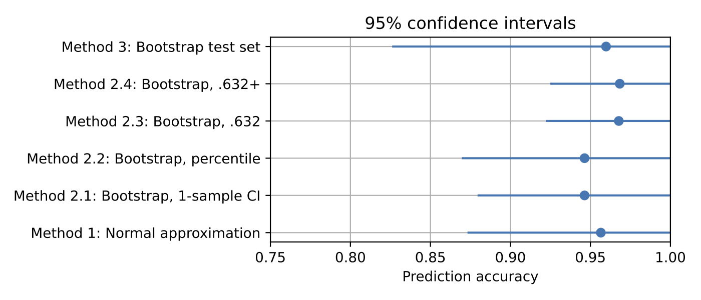
We can see that bootstrapping the test set results in the widest confidence intervals, and the .632 estimates result in the smallest confidence intervals. If the .632 confidence intervals are correct (contain the true parameter 95% of the time), these would be most desirable from an accuracy standpoint.
Slimmer 95% confidence intervals are desirable because they narrow down the possible range for the actual parameter value we are estimating. However, this is only so far useful as the confidence interval method is accurate. How do we know which way is actually correct or precise? That’s hard to probe with real datasets because the amount of data in real datasets is limited. Otherwise, it would not be necessary to construct confidence intervals in the first place.
However, which confidence interval methods are correct or are most accurate is tricky to answer. The following section describes an analysis to look into this further.
Confidence Intervals and the True Model Performance
Let’s look at the results of a small simulation study to investigate how precise the different confidence interval methods are. Here, we are interested in seeing whether the true model accuracy (generalization accuracy) is actually contained in the confidence intervals.
We create a synthetic dataset consisting of 10 million and 2 thousand data points for classification. The first 1000 data points are used for training, the second 1000 data points are used for testing, and the remaining 10,000,000 data points represent the dataset we use to calculate the model’s true performance.
(A Jupyter notebook containing the code examples for this simulation study be found here.)
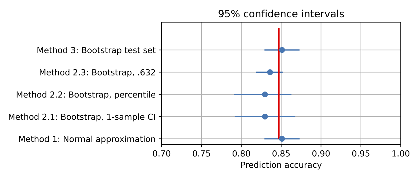
The red vertical line indicates the true accuracy of the model as evaluated on the 10 million test data points. We omitted two methods from this graph: method 4, as the random seeds don’t affect the decision tree model, and method 2.4, as the .632+ bootstrap method is too computationally expensive for this dataset.
As we can see, all 95% confidence interval methods contain the true parameter, which is good. Moreover, the “bootstrapping the test set” (method 3) and “normal approximation” (method 1) methods yield average accuracy estimates that are closest to the true accuracy, which is a nice bonus.
However, this simulation study should be taken with a grain of salt: changing the amount of label noise in the dataset can result in noticeably different outcomes. Also, ideally, we want to repeat this simulation many times and see if the confidence intervals contain the true parameter 95% of the time. I originally wanted to leave this as an exercise to the reader. Still, then I couldn’t resist running this experiment here.
Below are the results from repeating the above simulation study 1,000 times with different random seeds for generating the synthetic datasets:
| Method | Number of times 95% CI contains the true accuracy | |
|---|---|---|
| 1 | Normal approximation | 95.6% |
| 2.1 | Bootstrap, 1-sample CI | 98.5% |
| 2.2 | Bootstrap, percentile | 98.0% |
| 2.3 | Bootstrap, .632 | 83.2% |
| 3 | Bootstrap test set | 94.5% |
The normal approximation (method 1) and test set bootstrap (method 3) are the most precise methods, as approximately 95% of their 95% confidence intervals contain the true accuracy. On the other hand, methods 2.1 and 2.2 appear too conservative (the confidence intervals are wider than need be), and the .632 bootstrap method seems to yield incorrect results, either because the confidence intervals are too narrow or biased (shifted too much).
Conclusion
Both the normal approximation (method 1) and bootstrapping the test sets (method 3) are practical and accurate options. When it comes explicitly to deep learning models, considering different random seeds (method 4) is another technique worth considering. Note that both methods 1 and 2 are convenient as they don’t require training multiple models, unlike method 4. However, method 4 might be attractive for algorithm comparisons as it also tells us how dependent an algorithm is on the random seed. In deep learning, this is especially important because sometimes a method can look worse than it really is if we pick an unlucky random seed (and vice versa).
This article mainly focuses on giving you an overview of the different confidence methods as well as some pros and cons. For example, some estimate the uncertainty by varying the test sets, some by varying the random seeds. Given the amount of computing resources available, combining multiple methods (e.g., out-of-bag bootstrapping or test set bootstrapping and changing the learning algorithm’s random seed) may be other avenues to consider. For instance, in the aforementioned Accounting for variance in machine learning benchmarks study, the researchers found that randomizing as many sources of variation as possible can help reduce the estimation error.
Also, as mentioned at the beginning of the article, confidence intervals are only one way to communicate uncertainty. Machine learning benchmark studies don’t necessarily have to be accompanied by confidence intervals. More straightforward statistics such as the variance or standard deviation across multiple repetitions can already be helpful for both readers and reviewers.
Bonus: Creating Confidence Intervals with TorchMetrics
In the context of deep learning and PyTorch, I recently wrote about TorchMetrics, a nice tool for evaluating models in cases where the dataset is too large to fit into memory. While the above-listed code for bootstrapping the test set (method 3) is relatively straightforward, you may be interested in using TorchMetrics for this job.
For comparison, the code for bootstrapping the test set we used earlier was as follows:
In:
clf.fit(X_train, y_train)

predictions_test = clf.predict(X_test)
acc_test = np.mean(predictions_test == y_test)

rng = np.random.RandomState(seed=123)
idx = np.arange(y_test.shape[0])

test_accuracies = []

for i in range(200):

    pred_idx = rng.choice(idx, size=idx.shape[0], replace=True)
    acc_test_boot = np.mean(predictions_test[pred_idx] == y_test[pred_idx])
    test_accuracies.append(acc_test_boot)

bootstrap_train_mean = np.mean(test_accuracies)
bootstrap_train_mean
Out:
0.956304347826087
In:
ci_lower = np.percentile(test_accuracies, 2.5)
ci_upper = np.percentile(test_accuracies, 97.5)

print(ci_lower, ci_upper)
Out:
0.8695652173913043 1.0
Using the Bootstrapper from TorchMetrics, we can we can replicate the results from above as follows:
In:
import torch
from torchmetrics import Accuracy, BootStrapper

torch.manual_seed(123)

quantiles = torch.tensor([0.05, 0.95])
base_metric = Accuracy()
bootstrap = BootStrapper(
    base_metric, num_bootstraps=200, sampling_strategy="multinomial", quantile=quantiles
)

bootstrap.update(torch.from_numpy(predictions_test), torch.from_numpy(y_test))
output = bootstrap.compute()

print(output)
Out:
{'mean': tensor(0.9602), 'std': tensor(0.0408), 'quantile': tensor([0.8696, 1.0000])}
Note that this can come in really handy in practice if we want to compute things incrementally (for example, if the test set is too big for memory). Let’s assume the predictions come in multiple chunks:
In:
idx = np.arange(predictions_test.shape[0])
groups = np.array_split(idx, 3)
In:
torch.manual_seed(123)

quantiles = torch.tensor([0.05, 0.95])
base_metric = Accuracy()
bootstrap = BootStrapper(
    base_metric, num_bootstraps=200, sampling_strategy="multinomial", quantile=quantiles
)

for group in groups:

    pred_chunk = torch.from_numpy(predictions_test[group])
    label_chunk = torch.from_numpy(y_test[group])

    bootstrap.update(pred_chunk, label_chunk)

output = bootstrap.compute()
print(output)
Out:
{'mean': tensor(0.9550), 'std': tensor(0.0421), 'quantile': tensor([0.8696, 1.0000])}
If you read the book and have a few minutes to spare, I'd really appreciate a brief review. It helps us authors a lot!
Your support means a great deal! Thank you!