Chapter 1: Introduction to Machine Learning and Deep Learning
Note: This is a write-up of the lecture slides I created for the deep learning class I am teaching at UW-Madison. You can find a recent version of these slides here: https://github.com/rasbt/stat453-deep-learning-ss20. Earlier this summer, I started a writing routine, writing ~25 minutes every morning at ~7 am when I woke up. This is the culmination of it so far. Maybe, one day, this will be a book. If you are reading this, I’d really appreciate your feedback. But please don’t be too harsh, since this is a first draft that hasn’t undergone any editing. (PS: Sorry, I also don’t know when the next chapter will be ready, it may be a long time. Also, I realize that there are countless introductions to machine learning and deep learning out there already; nonetheless, I cannot start a course or book without an introduction.)
I hope this is useful to you :).
Chapter 1: Introduction to Machine Learning and Deep Learning
“Beginning is easy – continuing is hard.” – Japanese Proverb
This first chapter introduces the core ideas and concepts of machine learning, before diving deeper into deep learning in the following chapters. First, we define what machine learning is and how it is related to traditional forms of automation, namely, programming. We then cover the three broad categories of machine learning: supervised learning, unsupervised learning, and reinforcement learning. Lastly, based on a typical predictive modeling pipeline, this chapter introduces the core terminology and notation used in the deep learning field and throughout this book.
1.1 What is Machine Learning?
Before focusing in on the field of deep learning, it is helpful to introduce the broader concepts of machine learning – deep learning is a subfield of machine learning, which is further illustrated in this chapter (Section 1.1.2). But before we get ahead of ourselves, let us delve into one of the motivations behind developing and using machine learning.
1.1.1 Automating the Traditional Programming Paradigm
Imagine we just finished building a really nice email client. We just made our (and every user’s) life a lot easier by adding new features for snoozing emails. However, email inboxes are still being filled with large amounts of spam. How can we implement a spam filter to improve this situation?
Unfortunately, defining the rules for recognizing spam is a process that is a rather challenging task for us humans1. If we cannot give a precise definition of what constitutes spam, how can we develop and code a set of rules in the email program? Maybe we can implement some simple rules, for example, emails with subject lines written in “ALL CAPS”. But after applying this filter to real-world inbox folders, we likely find a large number of false negatives (spam email not classified as spam). So, maybe we should go back to the drawing board and add some additional rules.
The previous paragraph outlines the traditional programming paradigm in the context of developing an email client. It is an excellent approach to developing certain features, but it is not ideal for others. For example, when implementing an email spam filter, there may be a more efficient way than defining rules based on our intuition. Rather than relying on our intuition alone, we could read and analyze thousands or millions of emails in a dataset and take notes about what these spam emails have in common and distinguishes them from regular email. While this is in the realm of possibility, this certainly sounds tedious, daunting, and error-prone. There must be a better way, namely, using machine learning.
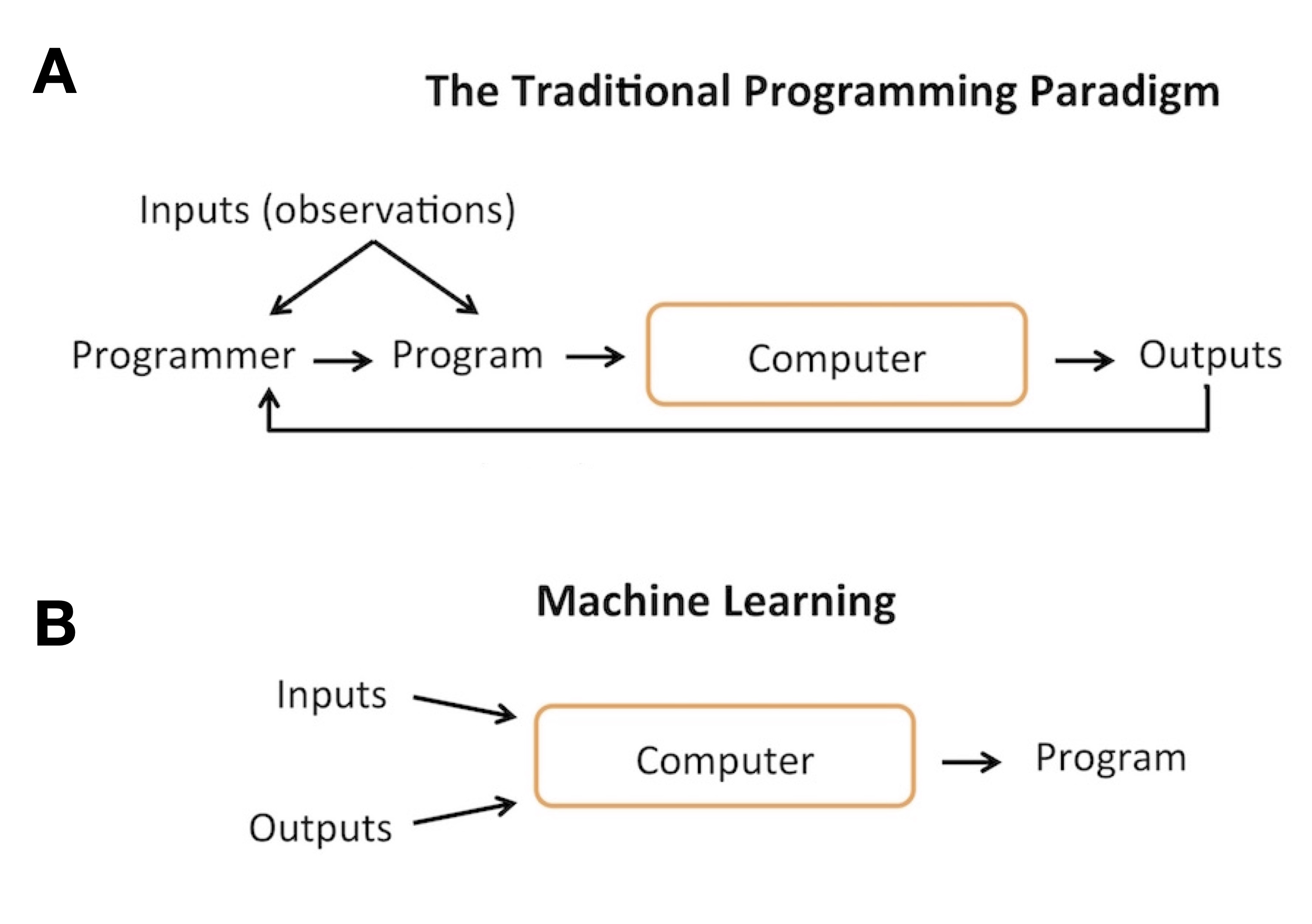 Figure 1. Comparison between traditional programming (A) and machine learning
(B).
Figure 1A describes the traditional programming paradigm where a programmer develops a set of rules or program, feeds it to the computer, and observes the output it produces. If the outputs are not satisfactory, the programmer goes back to the program and tweaks the rules in hope of improving the results (here: the number of correctly classified emails).
In contrast to the traditional programming paradigm, machine learning is about letting the computer figuring out such complex input-output relationships. As summarized in Figure 1B, the difference between the traditional programming paradigm and machine learning is that the latter is a paradigm that provides a computer algorithm with examples of the task we want to solve, and it will come up with the decision making “program” (here: machine learning model) that optimizes the decision making according to a user-defined objective.
1.1.2 The Connection between Machine Learning, Deep Learning, and AI
Artificial intelligence (AI) emerged as a subfield of computer science as the quest for programming computers to solve tasks that humans are good at (natural language, speech, image recognition, etc.). According to common belief, the term AI was first coined by John McCarthy at the Dartmouth Summer Research Project on Artificial Intelligence conference, a summer workshop that was held in 1956 [@emmertstreib2020clarification]. Eventually, the field of machine learning was created from the desire to design AI.
The first machine learning algorithms (Rosenblatt perceptrons, covered in Chapter 3, The Perceptron) were developed in the 1950s [@rosenblatt1958perceptron], inspired by early mathematical models of neurons in the human brain [@mcculloch1943logical]. In the following decades, neural networks with multiple neurons and layers were developed as well as algorithms to train them effectively [@rumelhart1986learning]. For reasons that are covered in greater detail in Chapter 2, A Brief Summary of the History of Neural Networks and Deep Learning, multilayer neural networks have seen a revival under the umbrella term deep learning around 2012.
Due to the increased focus on deep learning methods in the last decade, as well as the evolving technology stack and algorithmic techniques, the branch of machine learning that does not concern deep neural networks2 are now often referred to as traditional or conventional machine learning [@raschka2020machine].
As described by the above paragraphs, there is a close connection and overlap among the fields of machine learning, AI, and deep learning, as depicted in Figure 2. AI can be understood as the quest for developing non-biological systems that exhibit human-like forms of intelligence. Early and promising approaches included symbolic models and reasoning, early versions of neural networks, and expert systems [@emmertstreib2020clarification]. After several ups and downs, later in the 20th century, machine learning (with and without neural networks) emerged as one of the most promising directions towards developing such artificially intelligent systems. In a nutshell, machine learning is about teaching machines or computers how to learn from data without the need for humans to hand-code specific rules.
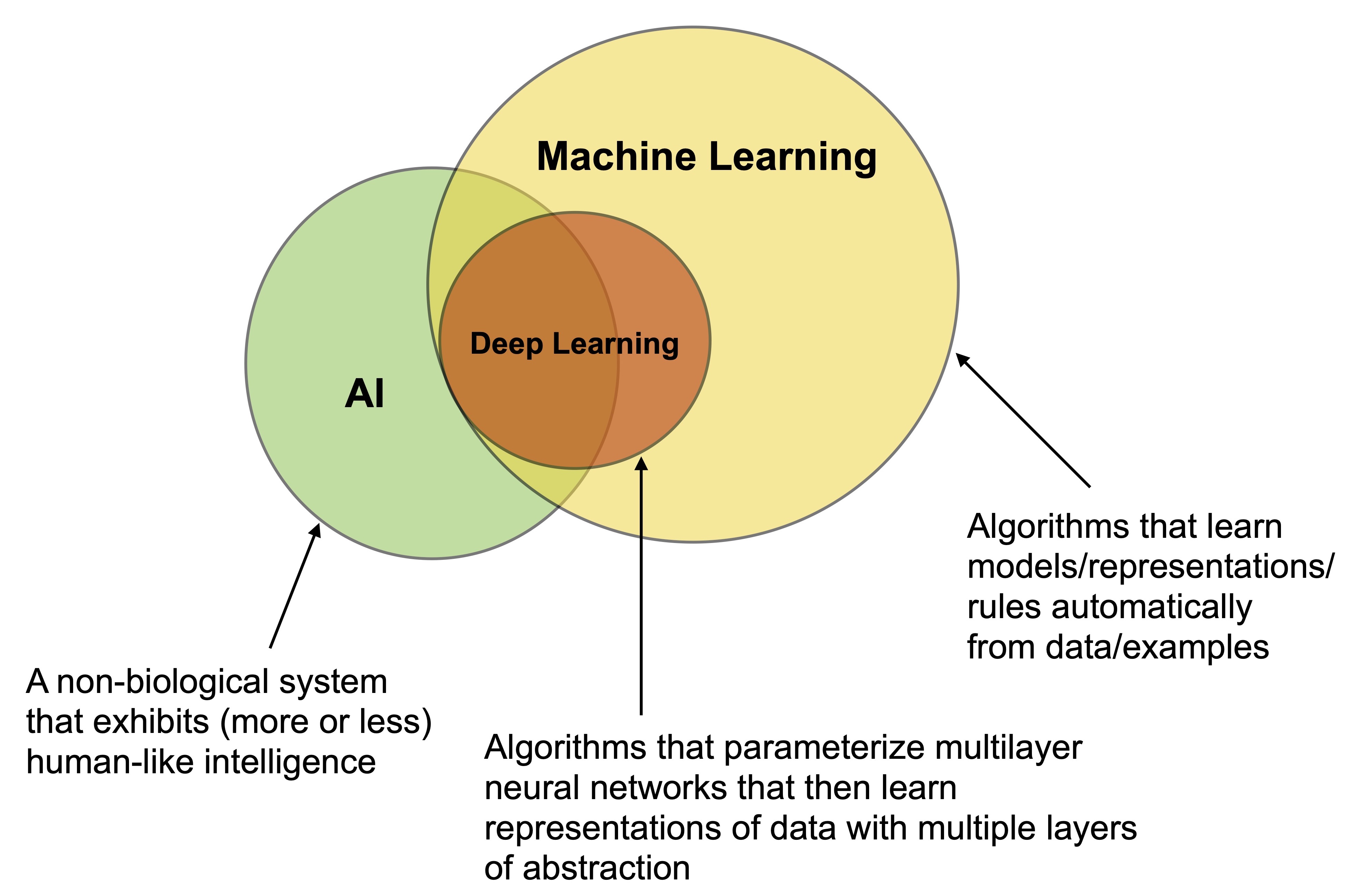 Figure 2. The close connection and overlap between the fields of machine
learning, deep learning, and artificial
intelligence.
While machine learning can be used to develop AI, not all machine learning applications can be considered AI. For instance, if someone implements a decision tree for deciding whether someone deserves a loan based on age, income, and credit score, we usually do not think of it as an artificially intelligent agent making that decision (as opposed to some “simple rules”).
Approaches to AI that are not based on machine learning include the symbolic representations or logic rules, which can be written or programmed by observing a human expert performing a particular task. Systems that are developed based on observing human experts are called expert systems. The symbolic approach to AI is now sometimes called “Good Old-Fashioned Artificial Intelligence” [@haugeland1989artificial]. From a programming perspective, one can think of such expert systems as complex computer programs with many (deeply nested) conditional statements (if/else statements).
AI can be further categorized into artificial general intelligence (AGI) and narrow AI. AGI is focused on the development of multi-purpose AI mimicking human intelligence across tasks. Narrow AI focuses on solving a single, specific task (playing a game, driving a car, and so forth). In 2018, Martin Ford published a book containing interviews with leading artificial intelligence researchers centered around the topic when AGI will finally emerge [@ford2018architects]. To the interested reader: The range of the 18 guesses was between 11 years from 2018 (2029) and 182 years from 2018 (2200). The average prediction was 81 from 2018, that is, 2099.
In sum, we can describe classic AI as a non-biological system that exhibits human-like forms of intelligence on one or multiple tasks. Machine learning is a field concerned with the development of algorithms that learn models, representations, and rules automatically from data.
1.2 The Categories of Machine Learning
This section describes and summarizes the three classical categories of machine learning: supervised learning, unsupervised learning, and reinforcement learning. In addition to these three main categories, this section introduces the two main subcategories of supervised learning: semi-supervised learning, which can be considered a mix between supervised and unsupervised learning, and self-supervised learning.
As described in Section 1.1.2, deep learning is a subcategory of machine learning focused on parameterizing multilayer neural networks that can learn representations of the data with multiple layers of abstractions. Throughout this book, we will use the term machine learning to refer to both traditional machine learning and deep learning.
Supervised learning is focused on predictive modeling tasks, that is, modeling the relationship between features extracted from the data and one or multiple target variables or labels. While supervised learning is based on labeled data, unsupervised learning aims to model the hidden structure in data without label information. Finally, reinforcement learning is concerned with developing reward systems to model complex decision processes and learning series of actions.
1.2.1 Supervised Learning
Supervised learning is concerned with predicting a target value given input observations. In machine learning, we call the model inputs “features”3). The target values that supervised models are trained to predict are also often called labels4. Supervised learning can be categorized into two major subcategories: regression analysis and classification. In regression analysis, the target values or labels are continuous variables (Figure 3A). In classification, the labels are so-called class labels, which can be understood as discrete class- or group-membership indicators (Figure 3B).
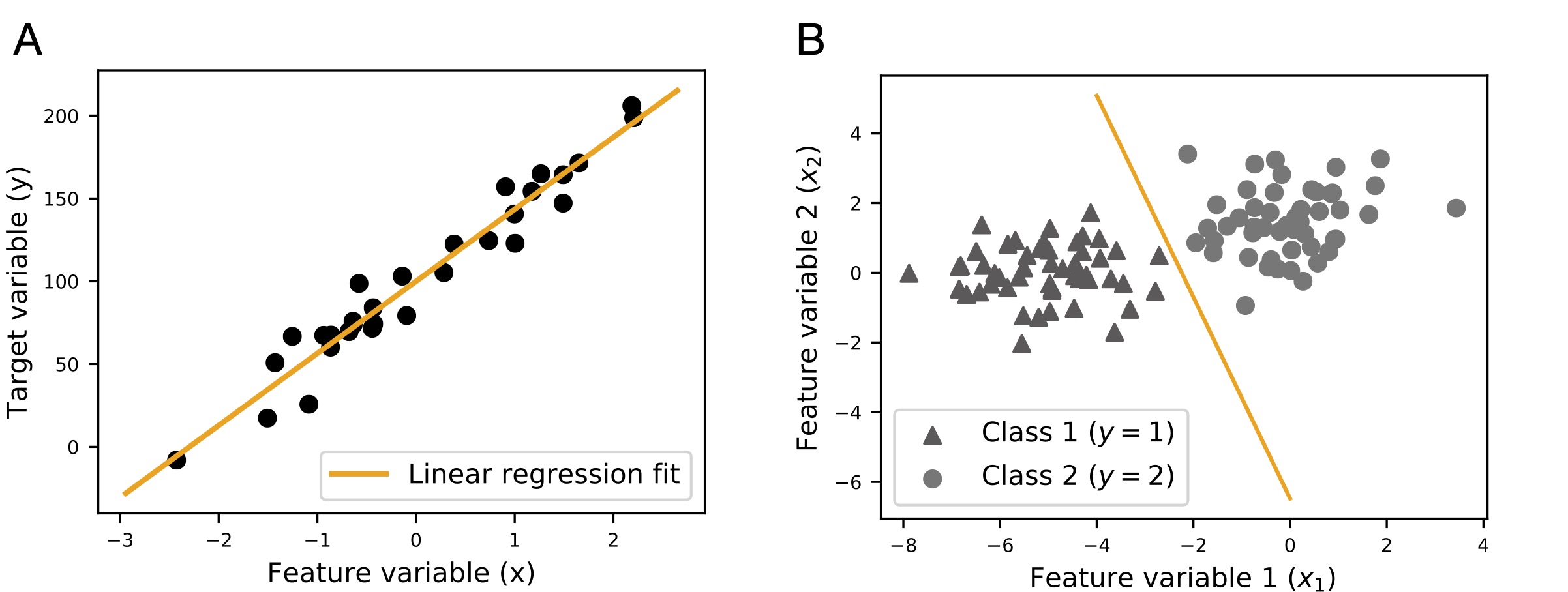 Figure 3. Illustrations of the two main categories of supervised learning,
regression (A) and classification
(B).
In machine learning, we often work with high-dimensional datasets; that is, datasets consisting of many input features. However, due to the limitations of the human imagination and the written medium, conventional illustrations can only depict two (or at most three) spatial dimensions. The 2D scatterplots in Figure 3 show two simple datasets. Here, sub-panel A depicts a simple regression example for a dataset with only a single feature. The target variable, the values we want to predict, is depicted as the y-axis. Sub-panel B depicts a 2-dimensional classification dataset, where the target variable, the discrete class label information, is encoded as a symbol (triangle vs. circle). In both cases, there is a target variable that the model learns to predict. In the case of the linear regression example, the target variable is a continuous variable depicted on the y-axis in Figure 3A. For the classification example in Figure 3B, the target variable is comprised of class labels depicted as symbols (triangles and circles).
The third category of supervised learning is ordinal regression, which is sometimes also referred to as ordinal classification. Ordinal regression can be understood as a hybrid between those as mentioned above, (metric) regression analysis and classification. In ordinal regression, we have categories just like in classification. However, there is ordering information between the classes. In contrast to metric regression, the labels are discrete, and the distance between the labels is arbitrary. For example, predicting a person’s height is an example of metric regression. The target variable (height) can be measured on a continuous scale, and the distance between 150 cm and 160 cm is the same as the distance between 180 and 190 cm. Predicting a movie rating on a 1-5 scale would be a better fit for an ordinal regression model. Assuming the movie rating scale is composed as follows: 1=bad, 2=ok, 3=good, 4=great, and 5=awesome. Here, the distance between 1 (bad) and 2 (ok) is arbitrary. Or in other words, we cannot directly compare the difference between 1 (bad) and 2 (ok) to the distance between 3 (good) and 4 (great). A task that is related to ordinal regression is ranking. However, note that in ranking, we are only interested in the relative order of the items. For example, we may order a collection of movies from worst to best. In ordinal regression, we care about the absolute values on a given scale. A detailed treatment of ordinal regression is out of the scope of this book. Readers interested in this topic may refer to the manuscript “Rank-consistent Ordinal Regression for Neural Networks” [@cao2019rank], which contains references to ordinal regression literature relevant to deep learning.
1.2.2 Unsupervised Learning
The previous section introduced supervised learning, which is the most prominent subcategory of machine learning. This section discusses the second major category of machine learning: unsupervised learning. In unsupervised learning, in contrast to supervised learning, no labeling information is given. The goal is to discover or model hidden structures in data rather than predicting continuous or discrete target labels.
One major subcategory of unsupervised learning is representation learning and dimensionality reduction. A popular and classic technique for this is principal component analysis (PCA; Figure 4).
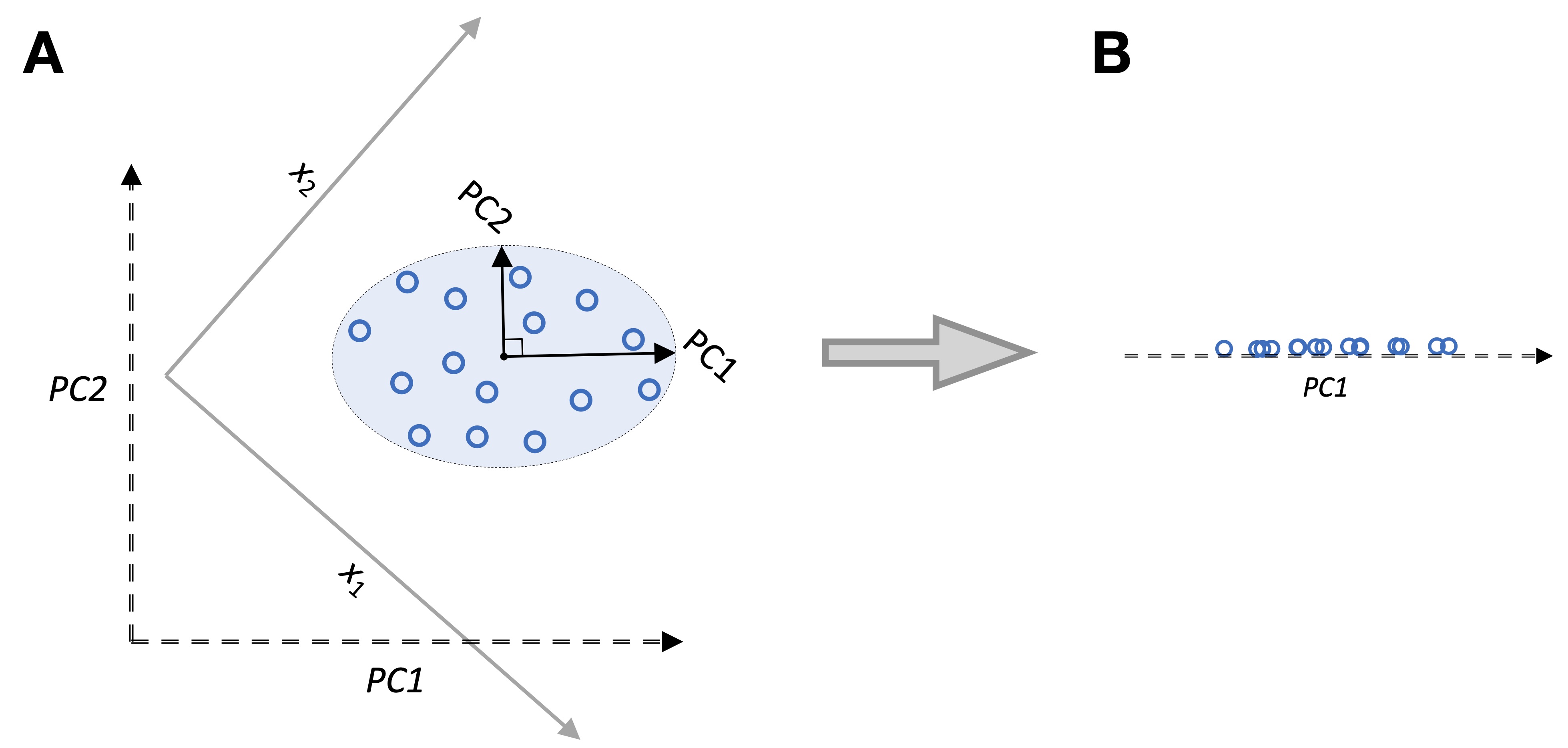 Figure 4. Illustrations of PCA. (A) A dataset (blue circles) with two feature
axis \(x_1\) and \(x_2\) that has been projected onto the principal
components \(PC1\) and \(PC2\) (B) A view of the data projected onto the
first principal component (PC1).
In a nutshell, PCA identifies the directions of maximum variance in a dataset. These directions (eigenvectors of the covariance matrix) form the principal component axes of a new coordinate system. In practice, PCA is typically used to reduce the dimensionality of a dataset while retaining most of its information (variance). PCA is a linear transformation technique. Thus, it cannot capture complex non-linear patterns in data; however, kernel PCA and other non-linear dimensionality reduction techniques exist. Chapter 15 covers autoencoders, which are deep neural network architectures that can be used for non-linear dimensionality reduction. An autoencoder consists of two subnetworks, an encoder and a decoder, as illustrated in Figure 5. An input (for example, an image) is passed to the encoder, which compresses the input into a lower-dimensional representation, also known as “embedding vector” or “latent representation.” After the encoder embedded the feature into this lower-dimensional space, the decoder reconstructs the original image from this latent representation. The two subnetworks, encoder and decoder, are connected end to end and often depicted as an hourglass where the width of the hourglass represents the size of the feature map produced by the multilayer neural network.
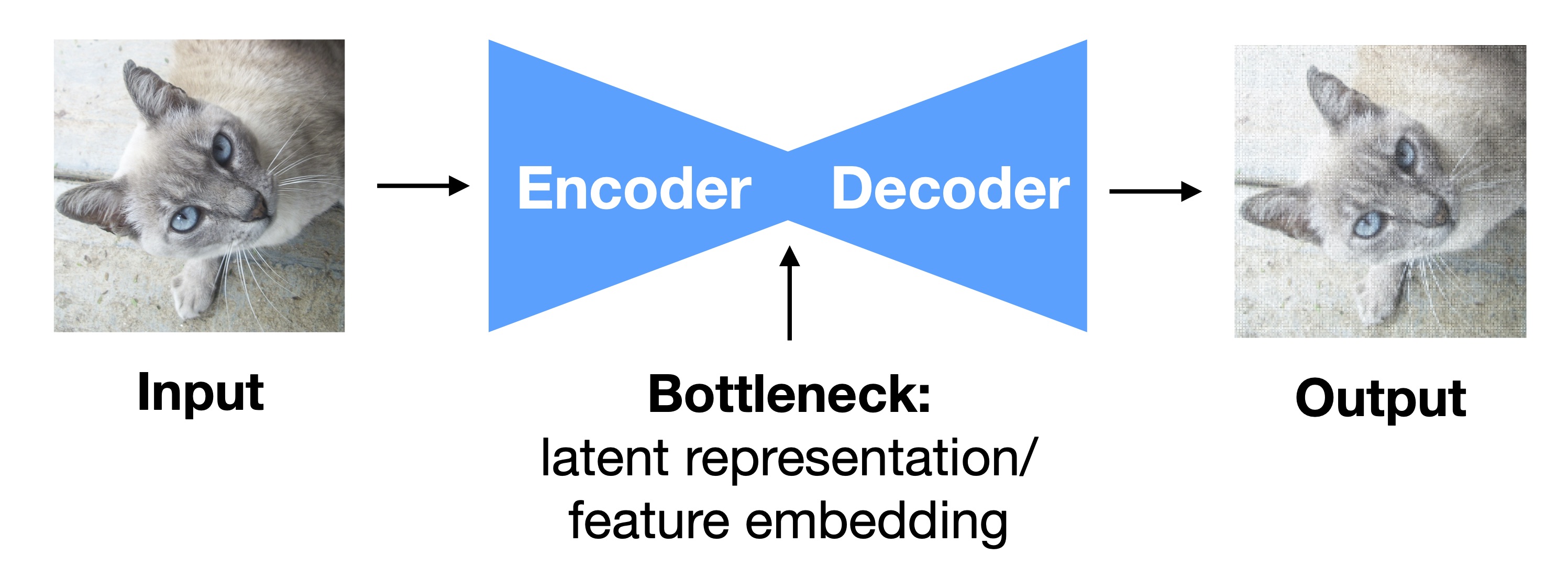 Figure 5. Illustration of an
autoencoder.
In a typical autoencoder architecture, the encoder’s output is the smallest feature map in the network, which is then fed into the decoder – this connection between encoder and decoder is also often referred to as the “bottleneck.” The rationale behind the autoencoder idea is that for the decoder to produce a faithful reconstruction of the original input image, the encoder must learn to create a latent representation that preserves most of the information. Typically, the autoencoder architecture is designed such that the latent representation is lower-dimensional than the input (and its reconstruction), so that the autoencoder cannot just memorize and pass the original input through the architecture – this is sometimes also referred to as information bottleneck.
Another major subcategory of unsupervised learning is clustering, which assigns group membership information to data points. It can be thought of as a task similar to classification but without labeling information given in the training dataset. Hence, in the absence of class label information, the clustering approach is to group data records by similarity and define distinct groups based on similarity thresholds.
Clustering can be divided into three major groups: prototype-based, density-based, and hierarchical clustering. In prototype-based clustering algorithms, such as K-Means [@macqueen1967some; @lloyd1982least], a fixed number of cluster centers is defined (the cluster centers are repositioned iteratively), and data points are assigned to the closest prototype based on a pair-wise distance measure (for example, Euclidean distance). In density-based clustering, unlike in prototype-based clustering, the number of cluster centers is not fixed but assigned by identifying regions of high density (the location of many data records close to each other measured by a user-defined distance metric. In hierarchical clustering, a distance metric is used to group examples in a tree like-fashion, where examples at the root are more related to each other. The depth of the tree defines the number of clusters.
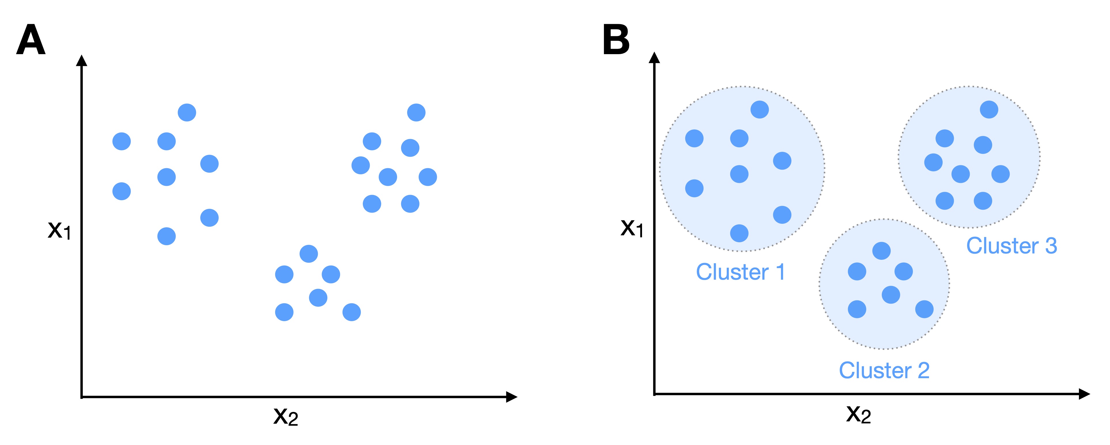 Figure 5. Illustration of clustering. (A) A two-dimensional, unlabeled dataset.
(B) Clusters inferred by a clustering algorithm that groups similar
points into the same
cluster.
1.2.3 Reinforcement Learning
The third and probably most challenging subcategory of machine learning is reinforcement learning (Figure 6). In contrast to supervised learning, which focuses on predicting a specific outcome, reinforcement learning is concerned with learning a series of actions that lead to a particular outcome. To illustrate reinforcement learning in the context of Figure 6, (1) given a chess board state \(S_t\)and some reward value \(R_t\) at iteration \(t\), (2) the reinforcement learning agent selects an action \(A_t\) that moves one of the pawns by two fields. (3) Next, the environment considers \(A_t\) to produce the next state, \(S_{t+1}\) and the corresponding reward for performing the action, \(R_{t+1}\). This cycle repeats until the end of the episode.
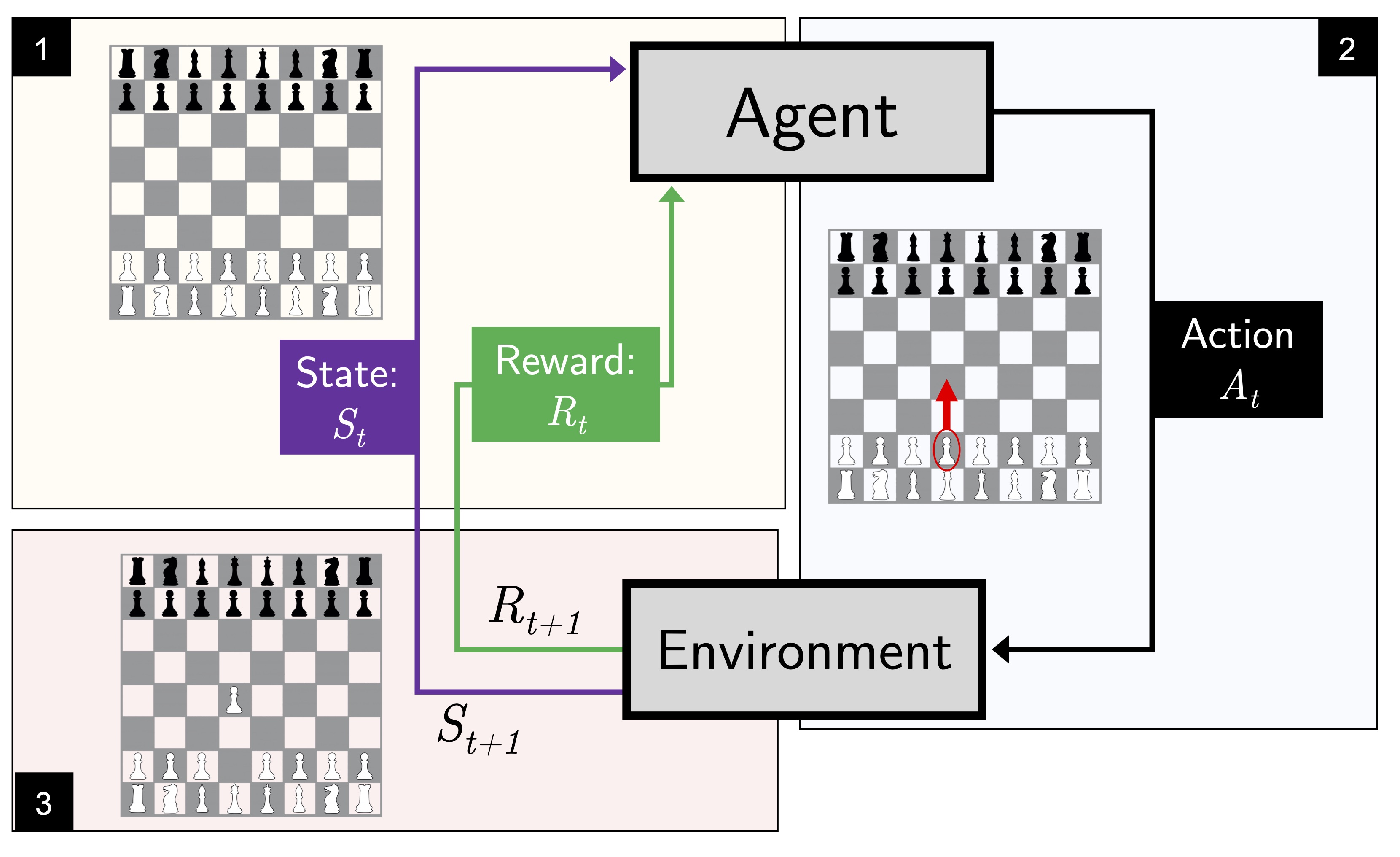 Figure 6. Illustration of reinforcement learning using a chess board as an
example.
1.2.4 Semi-supervised
Semi-supervised5 learning is a category mix between supervised and unsupervised learning. Semi-supervised learning refers to scenarios where some training examples are labeled while others are not. The main idea behind semi-supervised learning is to use the labeled portion of the dataset (via supervised learning) to label the unlabeled portion, which can then be used for supervised learning. Here, the use of unlabeled examples can improve generalization performance, as more data is available during training.
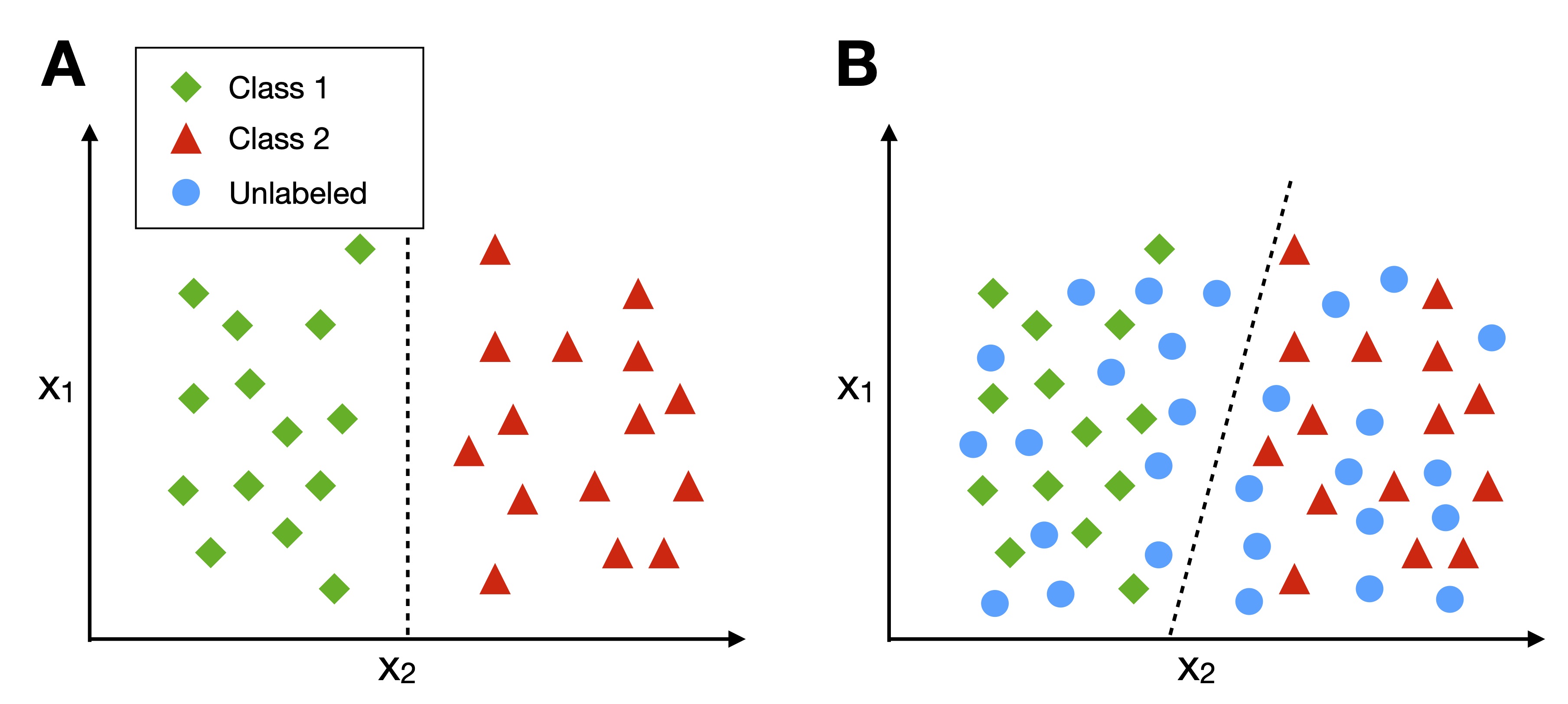 Figure 7. Illustration of semi-supervised learning incorporating unlabeled
examples. (A) A decision boundary derived from the labeled training
examples only. (B) A decision boundary based on both labeled and
unlabeled examples.
1.2.5 Self-supervised Learning
Collecting labels for large datasets can be prohibitively expensive. Self-supervised learning aims to leverage large amounts of unlabeled data for supervised learning. Due to its ability to use naturally available information as labels for supervised learning, self-supervised learning is sometimes also described as autonomous supervised learning. Both supervised learning and self-supervised learning are closely related since both learn mappings from inputs (for example, images) to outputs (for example, class labels) from labeled inputs-output pairs. What distinguishes self-supervised learning from regular supervised learning is that in the former, the labels are automatically generated or naturally embedded in the data.
Using self-supervised learning, a model (for supervised learning on a target task) can be (pre-)trained on a related task first, before it is trained on the target task. This allows leveraging more data. The related task is also often known as a “pretext task.” For image classification, common pretext tasks include predicting by how many degrees an image was rotated [@gidaris2018unsupervised], colorizing grayscale versions of an image [@zhang2016colorful], and reassembling an image that has been divided into subregions (somewhat similar to a jigsaw puzzle) [@noroozi2016unsupervised], or predicting the context of a random image patch [@doersch2015unsupervised] (Figure 8).
In practice, self-supervised learning is often used when the labeled dataset corresponding target task is relatively small, or the model could benefit from additional data. In this scenario, one could leverage a more extensive, unlabeled dataset of a similar type as the data for the target task (for example, images with the same resolution) and create the labels for the pretext task, as described in the previous paragraph. After pre-training the model (typically a neural network) on the pretext labels, it can be trained on the target-task dataset. In practice, pre-training a model on the pretext task can result in better model performance than training the model on the target-task dataset alone.
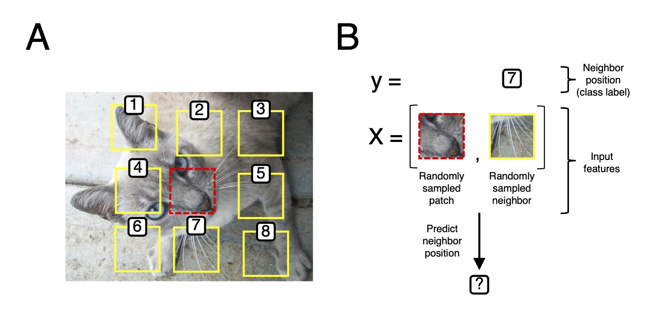 Figure 8. Self-supervised learning via context prediction. (A) A random patch is
sampled (red square) along with 9 neighboring patches. (B) Given the
random patch and a random neighbor patch, the task is to predict the
position of the neighboring patch relative to the center patch (red
square).
1.3 Machine Learning Terminology and Notation
Machine learning and deep learning research are very interdisciplinary. Depending on the researcher’s department or main area of expertise (statistics, computer science, or electrical engineering, and many others), the terminology primarily relies on their educational background. However, over the years, machine learning conferences and publishing venues converge to a field-specific terminology, jargon, and notation, which becomes more and more widely adopted within subfields.
1.3.1 Predictive Modeling Pipeline
For the most part, supervised learning is focused on developing predictive models; that is, training classifiers or regression models to predict target information (for instance, class labels) of new observations. The flowchart in Figure 9 summarizes a typical predictive modeling workflow, and details about certain aspects of this flowchart are covered in more detail in the following subsections.
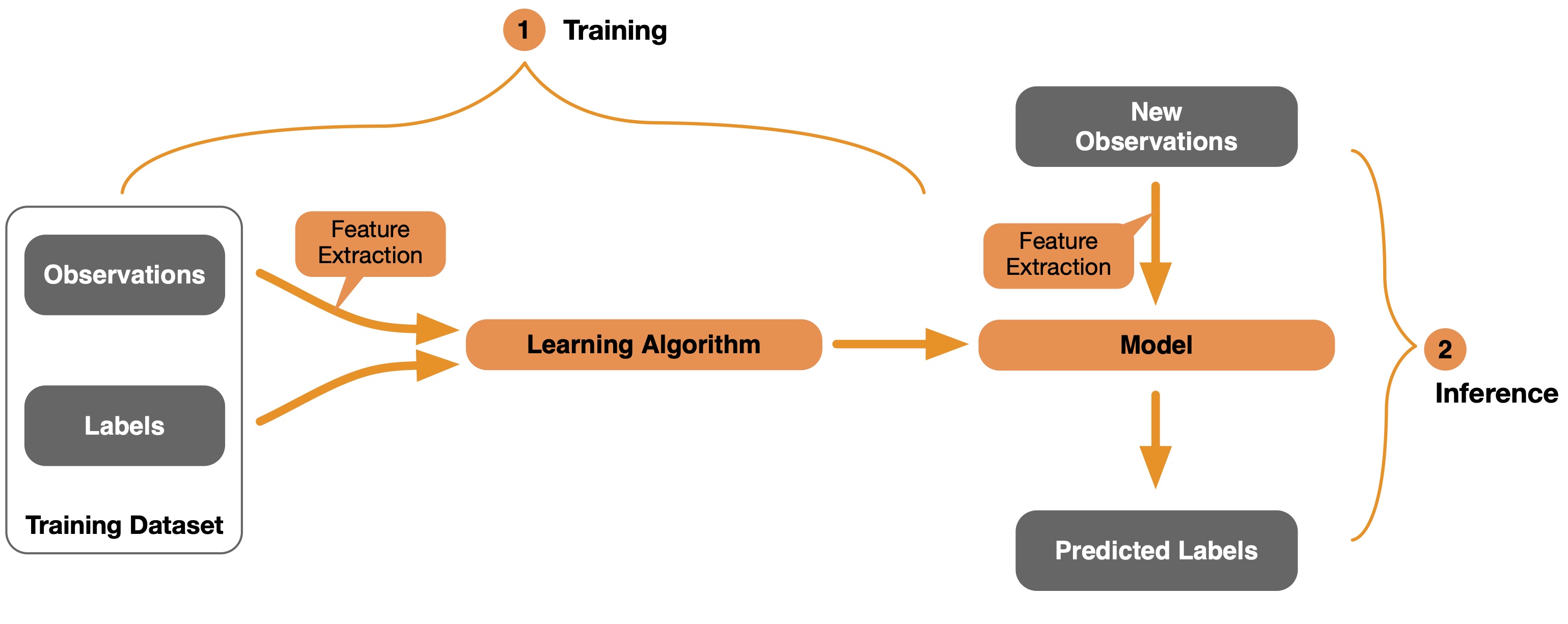 Figure 9. Illustration of a supervised learning and predictive modeling
pipeline.
In brief, the supervised learning workflow depicted in Figure 9 can be structured into two main steps: (1) model training and (2) inference. Training involves a labeled training dataset and a machine or deep learning algorithm. The learning algorithm learns how to associate the observations (also called features) in the training dataset – for example, images of flowers – with label information, such as the names of the flower species. In particular, the learning algorithm will use the training dataset to create or parameterize a predictive model that can then be used to make predictions on new observations.
Note that certain learning algorithms work on so-called “raw features” whereas other classes of learning algorithms operate on preprocessed or extracted features, which is discussed in more detail in the next subsection (Section 1.3.2).
Using a model to predict the target information of new observation is nowadays also called “inference”6 among deep learning researchers and practitioners. In practice, before we apply the model in the real world, we typically involve a model evaluation step. This is similar to the “inference” stage shown in Figure 9, but the new observations come from an independent test dataset for which we know the true labels that we want to predict. This basic model evaluation is illustrated in Figure 10: We apply the model to the new observations (data records from the test dataset) and then compare the predicted labels to the actual labels from the test dataset and compute an evaluation metric such as prediction error or accuracy. Note that model evaluation is a broad topic in itself that is out of the scope of this book. However, if you are interested in further details, I recommend the freely available article “Model Evaluation, Model Selection, and Algorithm Selection in Machine Learning” [@raschka2018model].
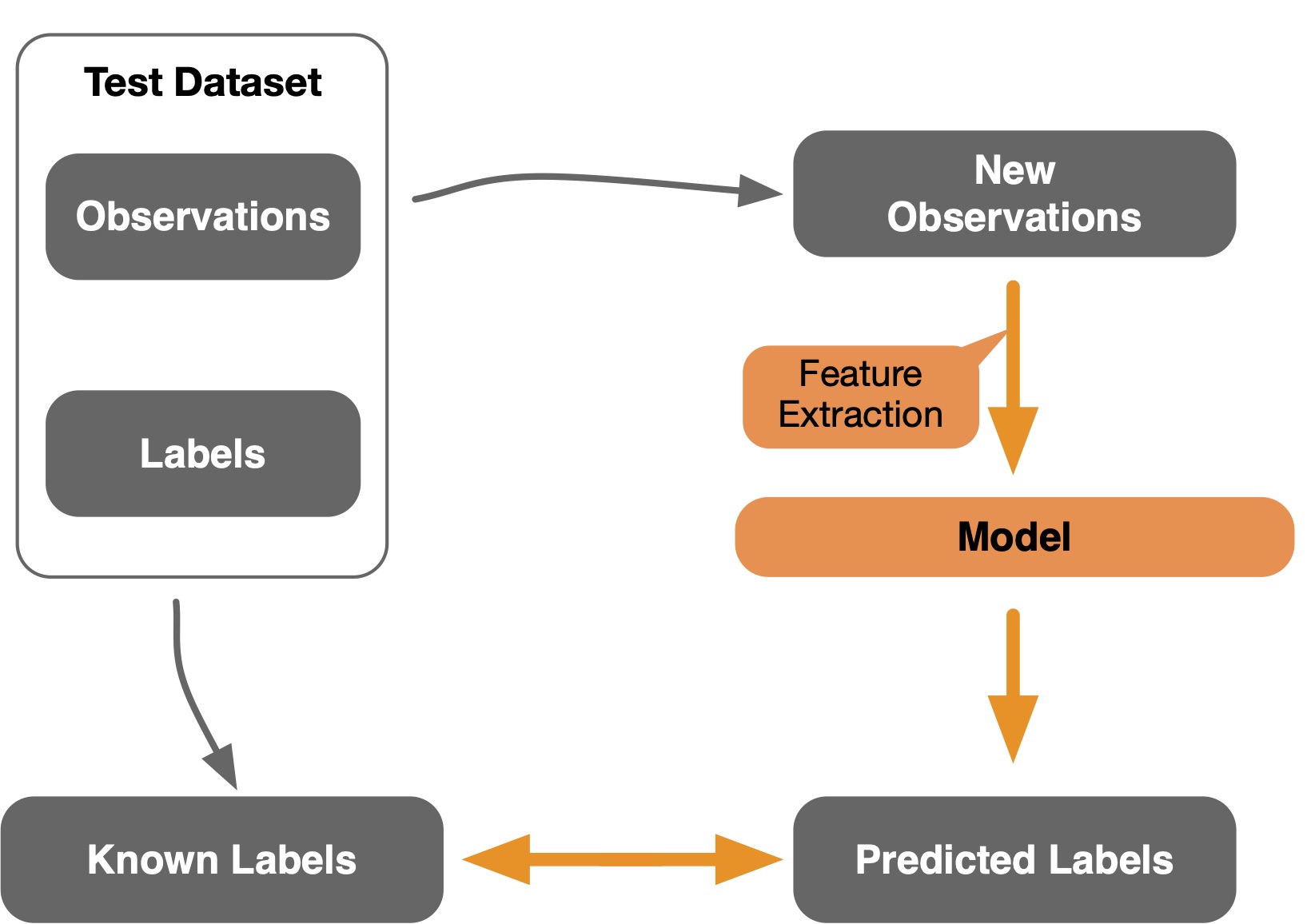 Figure 10. Using a test dataset to evaluate the performance of a predictive
model.
1.3.2 Data Representation
In the context of feature representation used in conventional machine learning versus deep learning, it is helpful to think about the concepts of structured and unstructured data (Figure 11).
In simple words, structured data can be understood as tabular data. A characteristic of structured data is that it usually has undergone preprocessing, including feature extraction. For example, structured data is typically stored in the form of database entries, spreadsheets, or CSV files. In machine learning, it is common to format structured data such that each row of the tabular dataset represents a data instance or record (for example, a training example). Each column represents an observed or extracted feature. In statistics, this type of data representation is also often referred to as design matrix. Figure 11 illustrates an example of a structured dataset containing iris flower leaf measurements (sepal length, sepal width, petal length, and petal width). Here, the first column is simply a dataset index. Columns 2-5 are the flower measurements (features) and comprise the design matrix component of the dataset. The last column contains the class label (here, the flower species: Iris-setosa, Iris-versicolor, and Iris-virginica) associated with each flower (training example). In a supervised learning setting, we could train a classifier to predict the class label (last column) from the features (columns 2-5).
Unstructured data described data closer to its raw form – the form that it was collected. For example, in the context of the iris flower example described in the previous paragraph, an unstructured data format would be a collection of images corresponding to the flowers listed in the structured dataset table shown in Figure 11A. It is then easy to see how features can be extracted from an unstructured data record (Figure 11B) to create a structured data record (a row in Figure 11A).
While machine learning is traditionally designed to work with structured data, deep learning has been developed with unstructured data in mind. Most deep learning architectures, such as convolutional and recurrent neural networks covered later in this book, are designed to operate on image and text data. As part of the learning process, deep neural networks learn to extract and transform the raw (unstructured) data such that it is conducive for predictive modeling (in supervised learning settings). For this reason, deep learning is also often described as representation learning.
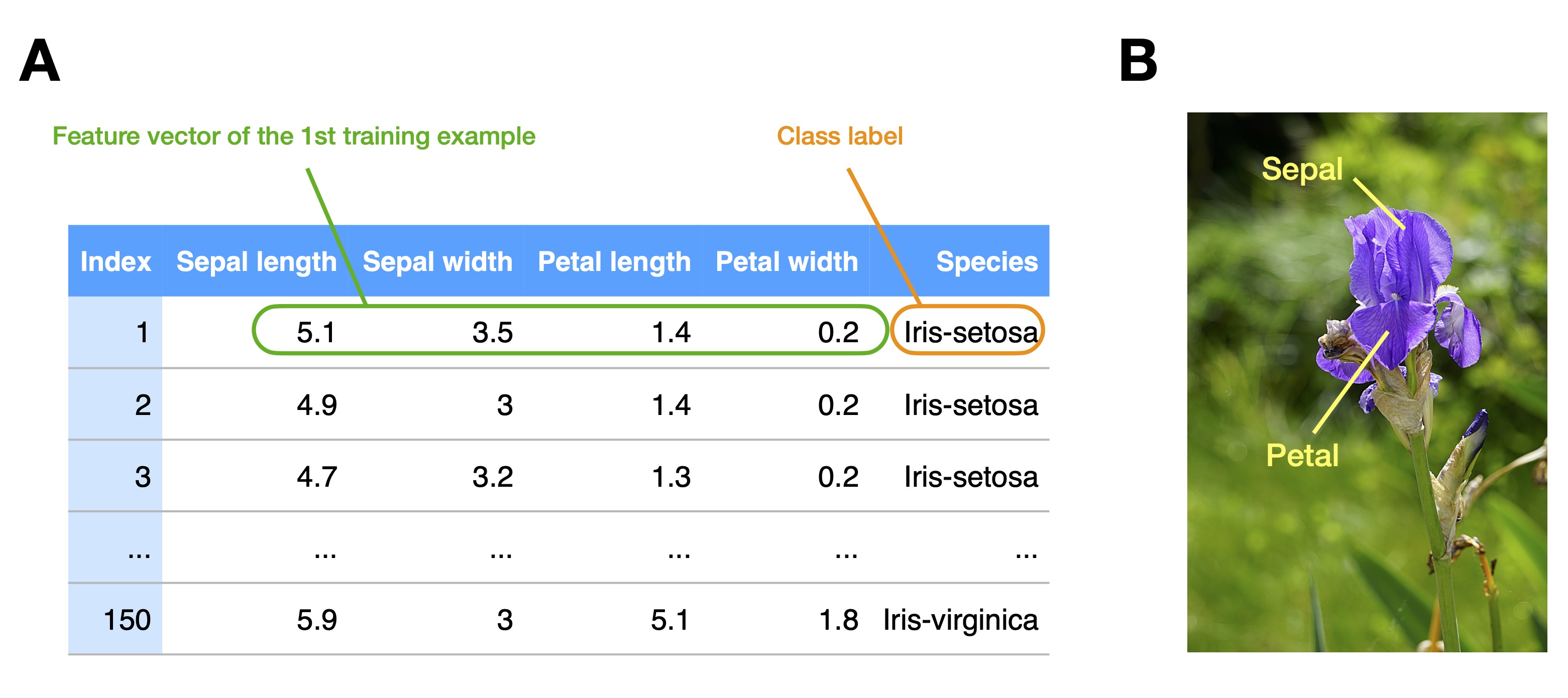 Figure 11. Structured versus unstructured data. (A) A structured, tabular dataset
for supervised learning where each row represents a training example
(here: iris flower) associated with four measurements and a class
label (iris species). (B) A photograph of an iris flower (unstructured
data). Such photographs can be processed into a structured dataset shown
in (A).
1.3.3 Supervised Learning Formalism
Recall Section 1.2.1, which introduced the largest subcategory of machine learning, supervised learning. More formally, we describe supervised learning as learning a function7 that maps an input space \(X\) to some output space \(Y\):
\[h: X \rightarrow Y.\]Given \(n\) labeled training examples, \(\mathcal{D} = \left\{\left(\mathbf{x}^{[1]}, y^{[1]}\right), \ldots,\left(\mathbf{x}^{[n]}, y^{[n]}\right)\right\}\), each training example, \(\left(\mathbf{x}^{[i]}, y^{[i]}\right)\) is a pair of inputs \(\mathbf{x}^{[i]}\) and label \(y^{[i]}\) (e.g., class label in classification). The inputs \(\mathbf{x}_{j}^{[i]\) are often referred to as features, and since \(\mathbf{x}^{[i]}\), represents a vector (in most traditional machine learning concepts), we usually refer to the inputs for a given training example as a feature vector:
\[\mathbf{x}=\left[\begin{array}{c} x_{1} \\ x_{2} \\ \vdots \\ x_{m} \end{array}\right].\]Given a feature vector for \(n\) training examples, we can represent the dataset (consisting of \(m\) features and \(n\) training examples) as a design matrix,
\[\mathbf{X}=\left[\begin{array}{c} \mathbf{x}_{1}^{\top} \\ \mathbf{x}_{2}^{\top} \\ \vdots \\ \mathbf{x}_{n}^{\top} \end{array}\right] = \left[\begin{array}{cccc} x_{1}^{[1]} & x_{2}^{[1]} & \cdots & x_{m}^{[1]} \\ x_{1}^{[2]} & x_{2}^{[2]} & \cdots & x_{m}^{[2]} \\ \vdots & \vdots & \ddots & \vdots \\ x_{1}^{[n]} & x_{2}^{[n]} & \cdots & x_{m}^{[n]} \end{array}\right].\]In the context of deep learning, where we often work with image data, the features (images) are higher-order tensors. This will be discussed in more detail in Chapter 4, Linear Algebra for Deep Learning and Chapter 12, Introduction to Convolutional Neural Networks.
1.3.4 Loss Function
Assuming some unknown, label generating function function \(f\) that associated the label \(y\) to the features \(\mathbf{x}\) in the \(i\)th training example, the goal of supervised learning is to learn a function \(h\) that can produce outputs or predictions \(\hat{y}\) for unlabeled datapoints \(\mathbf{x}\),
\[h(\mathbf{x}) = \hat{y}\]such that the predictive performance is optimized. In statistical learning theory, we express this as the minimization of risk \(R\), which we define as the expectation of a loss \(L\),
\[R(h)=E[L(h(x), y)]=\int L(h(x), y) d P(x, y).\]In supervised learning, the goal is to parameterize the model (i.e., find \(h\)) to minimize the risk. Since we do not know the joint probability distribution \(P(x, y)\) in practice, we resort to empirical risk minimization for all \(n\) examples in the given dataset:
\[R_{\mathrm{emp}}(h)=\frac{1}{n} \sum_{i=1}^{n} L\left(h\left(x_{i}\right), y_{i}\right).\]In machine learning literature, it is more common to denote the empirical risk \(R_{\mathrm{emp}}\), which is the sum of the loss over the training dataset (the lower, the better), as the cost function. Traditionally, the loss is a function that compares the predicted and actual labels for a single data record. For example, in classification, we can define the 0-1 loss as follows:
\[L(\hat{y}, y)_{\text{0-1}}=\delta(\hat{y} \neq y),\]where \(\delta\) is the Kronecker delta function
\[\delta({i \neq j}) \equiv\left\{\begin{array}{ll} 0 & \text{ for } i \neq j, \\ 1 & \text{ for } i=j. \end{array}\right.\]In regression, it is common to define a squared error loss,
\[L_{\text{SE}}(\hat{y}, y)=(\hat{y} - y)^2.\]Consequently, the mean squared error (MSE) measured over the entire dataset would be the cost function in this case:
\[\text{MSE}(h)=\frac{1}{n} \sum_{i=1}^{n} L_{\text{SE}}\left(h\left(x_{i}\right), y_{i}\right).\]Note that it was once common to distinguish between a loss function (single data record) and a cost function (loss function applied to the whole dataset) in machine learning literature. Deep learning literature largely abandoned this distinction or used the terms loss and cost interchangeably. In this book, however, we will distinguish between cost and loss function since it can enhance clarity and avoid unnecessary ambiguity.
Lastly, we shall note that in deep learning practice, it is usually not possible to optimize the 0-1 loss directly, so that we resort to surrogate functions for optimization purposes. For example, the categorical cross entropy measure serves as a surrogate for minimizing the prediction error (0-1 loss over the training set). This will be discussed in more detail in Chapter 5, Fitting Neurons with Gradient Descent. Broadly, what is important to remember is that there are (1) optimization performance measures and (2) evaluation measures – (1) and (2) can be the same but are often distinct (yet correlated). The ultimate goal is to achieve good performance concerning the evaluation measure or metric (for example, low classification error or high classification accuracy), which is highly correlated with optimizing the optimization measure, for example, the categorical cross entropy.)
1.3.5 A Glossary of Machine Learning Jargon
Machine learning has become a very interdisciplinary field. Researchers and practitioners from many disciplines, including computer science, statistics, neuroscience, mathematics, and several others, develop, shape, and contribute to the field. Consequently, depending on the researcher or practitioner’s background, different terms may be used to refer to similar concepts. This paragraph provides a quick overview of the most common machine and deep learning terms and their synonymous counterparts in other fields:
-
Training example. Synonymous to observation, training record, training instance, training sample (in some contexts, sample refers to a collection of training examples).
-
Feature. Synonymous to predictor, variable, independent variable, input, attribute, covariate.
-
Target. Synonymous to outcome, ground truth, desired output, response variable, dependent variable, label, class label (in the context of classification).
-
Output. Synonymous to model output or prediction; here, output means the return value of the model that is to be matched against the target.
1.4 Chapter Summary
This chapter introduced the core ideas (or desires) of machine learning and explained the relationship between machine learning, deep learning, and artificial intelligence. In sum, the takeaway is that deep learning is a subfield of machine learning, and artificial intelligence and machine learning are not synonyms. Moreover, this chapter introduced the three broad categories of machine learning, that is, working with labeled data (supervised learning) and unlabeled data (unsupervised learning), and learning complex processes (reinforcement learning). Ultimately, there is a lot of domain-specific jargon surrounding deep learning. A lot of technical terms are from other fields, but be aware that familiar terms may refer to something different in the context of deep learning.
The next chapter will delve deeper into the history of deep learning, introducing the broader ideas behind developing artificial neurons and neural networks. The next chapter aims to provide a top-down view of deep learning before we dissect it in a bottom-up fashion.
Thank you for reading. If you liked this content, you can also find me on Twitter, where I share more helpful content.
1.5 References
@cao2019rank: Cao, W., Mirjalili, V., & Raschka, S. (2019). Rank-consistent ordinal regression for neural networks. arXiv:1901.07884.
@doersch2015unsupervised: Doersch, C., Gupta, A., & Efros, A. A. (2015). Unsupervised visual representation learning by context prediction. In Proceedings of the IEEE International Conference on Computer Vision (pp. 1422-1430).
@emmertstreib2020clarification: Emmert-Streib, F., Yli-Harja, O., & Dehmer, M. (2020). A clarification of misconceptions, myths and desired status of artificial intelligence. arXiv:2008.05607.
@ford2018architects: Ford, M. (2018). Architects of Intelligence: The truth about AI from the people building it. Packt Publishing Ltd.
@gidaris2018unsupervised: Gidaris, S., Singh, P., & Komodakis, N. (2018, April). Unsupervised representation learning by predicting image rotations. In ICLR 2018.
@haugeland1989artificial: Haugeland, J. (1989). Artificial intelligence: The very idea. MIT Press.
@lloyd1982least: Lloyd, S. (1982). Least squares quantization in PCM. IEEE Transactions on Information Theory, 28(2), 129-137.
@macqueen1967some: MacQueen, J. (1967, June). Some methods for classification and analysis of multivariate observations. In Proceedings of the fifth Berkeley symposium on mathematical statistics and probability (Vol. 1, No. 14, pp. 281-297).
@mcculloch1943logical: McCulloch, W. S., & Pitts, W. (1943). A logical calculus of the ideas immanent in nervous activity. The Bulletin of Mathematical Biophysics, 5(4), 115-133.
@noroozi2016unsupervised: Noroozi, M., & Favaro, P. (2016, October). Unsupervised learning of visual representations by solving jigsaw puzzles. In European Conference on Computer Vision (pp. 69-84). Springer, Cham.
@raschka2018model: Sebastian Raschka (2018). Model Evaluation, model selection, and algorithm selection in machine learning. arXiv:1811.12808
@raschka2020machine: Raschka, S., Patterson, J., & Nolet, C. (2020). Machine Learning in Python: Main developments and technology trends in data science, machine learning, and artificial intelligence. Information, 11(4), 193.
@rosenblatt1958perceptron: Rosenblatt, F. (1958). The perceptron: a probabilistic model for information storage and organization in the brain. Psychological Review, 65(6), 386.
@rumelhart1986learning: Rumelhart, D. E., Hinton, G. E., & Williams, R. J. (1986). Learning representations by back-propagating errors. Nature, 323(6088), 533-536.
@zhang2016colorful: Zhang, R., Isola, P., & Efros, A. A. (2016, October). Colorful image colorization. In European Conference on Computer Vision (pp. 649-666). Springer, Cham.
1.6 Acknowledgements
I would like to thanks Andrea Panizza for useful feedback on the manuscript.
1.7 Footnotes
This blog post was exported from a LaTeX document, I apologize for the clumsy formatting and footnote handling.
-
If you disagree, try answering the question “What constitutes spam?” and apply the criteria to your inbox and spam folders. ↩
-
This includes nearest neighbor algorithms, generalized linear models, support vector machines, decision trees, random forests, and many others. ↩
-
Features are equivalent to the terms predictor variables, independent variables, or covariates used in statistics. ↩
-
This is the independent variable or outcome in statistics. ↩
-
The prefix semi- was borrowed from Latin and means “half.” ↩
-
The usage of the word “inference” in deep learning is not to be confused with its meaning in statistics, where it refers to the process of inferring information about a population based on sample statistics. ↩
-
While the exact symbol is not important, in machine learning, the letter \(h\) is often used to refer to the model or classifier. In this context, \(h\) is short for hypothesis. The hypothesis, in the context of a classification model, is a function that predicts a class label, thereby approximating the true, underlying function or phenomena determining the class label associated with a set of observations (features). ↩
If you read the book and have a few minutes to spare, I'd really appreciate a brief review. It helps us authors a lot!
Your support means a great deal! Thank you!